Method 1 – Using STOCKHISTORY Function to Gather Historical Data of NSE Stocks in Excel
Determine the stock data for the following companies of NSE every month from 1/1/2022 to 5/26/2022 (today’s date and format is m/dd/yyyy).

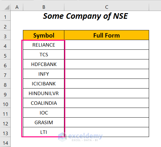
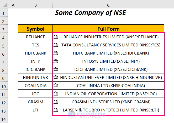
Step-01: Getting Full Names of Companies from Symbols
- To show the details of the symbols of the companies, an extra column, Full Form, has been added to accommodate the full names of the companies.
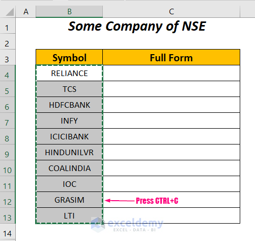
- Press CTRL + C to Copy the symbols of the companies.
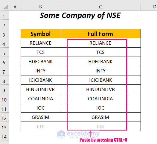
- The copied symbols will be pasted into the Full Form column by pressing CTRL + V
- To convert the symbols to the full name of the companies, select the Full Form range and then go to the Data Tab >> Data Types Group >> Stocks Option.
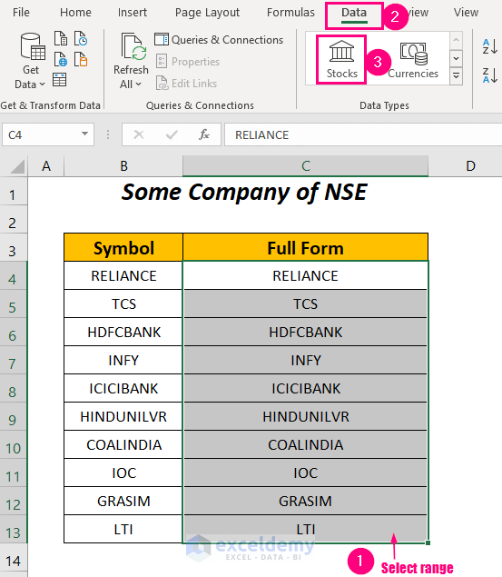
Get the Full form of the companies.
Step-02: Creating Basic Outline to Gather Historical Data of NSE Stocks in Excel
Use the symbols of the companies due to brevity and then add 5 extra columns to accumulate the stock data for these companies for 5 months.
We kept 2 cells for inserting the date limits; Starting Date and Closing Date.

- Write down the starting date from which you want the historical data (here, we used 1/1/2022).

- Using the TODAY function, you can set the closing date in cell H6.
=TODAY()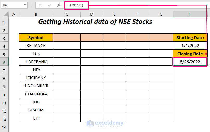
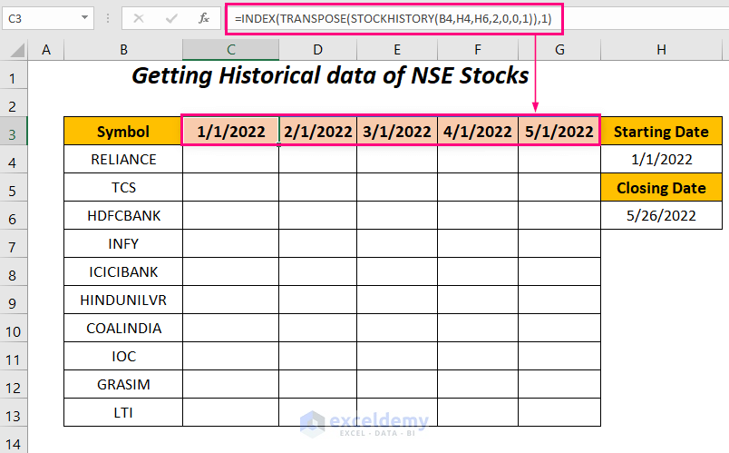
Step-03: Using Formula to Retrieve Stock Data
- We want the dates of each month as the header of the stock values, so used the following formula in cell C2.
=INDEX(TRANSPOSE(STOCKHISTORY(B4,H4,H6,2,0,0,1)),1)STOCKHISTORY(B4, H4, H6, 2, 0, 0,1) → B4is the symbol of the company,H4is the starting date,H6is the closing date,2is the interval asMonthly(0→Daily,1→Weekly,2→Monthly),0is forno headers, the second0is for the property asDate,1is the second property forClose. It will return the dates along with the stock values.
Output →{44562,2386.6; 44593,2359.55; 44621,2634.75; 44652,27990.25; 44682,2612}
TRANSPOSE(STOCKHISTORY(B4, H4, H6, 2, 0, 0,1))becomes
TRANSPOSE({44562,2386.6; 44593,2359.55; 44621,2634.75; 44652,27990.25; 44682,2612}) →The TRANSPOSE functiontransposes the date values because we want to gather the dates horizontally here for each company.
Output →{44562, 44593, 44621, 44652, 44682; 2386.6,2359.55,2634.75,27990.25,2612}
INDEX(TRANSPOSE(STOCKHISTORY(B4,H4,H6,2,0,0,1)),1)becomes
INDEX({44562, 44593, 44621, 44652, 44682; 2386.6,2359.55,2634.75,27990.25,2612},1) →returns the first array with dates among the two arrays for the dates and stock values.
Output →1/1/2022

After pressing ENTER, you will get the following 5 dates for each month.
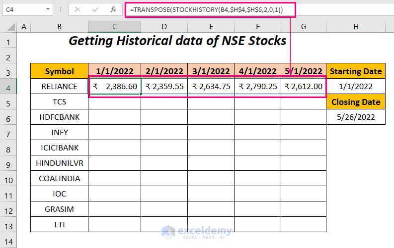
- To extract the stock values for RELIANCE, use the following formula in cell C4.
=TRANSPOSE(STOCKHISTORY(B4,$H$4,$H$6,2,0,1))STOCKHISTORY will return the monthly closing stock values for the RELIANCE company, and then TRANSPOSE will reverse the column values into rows to align horizontally with the company name.
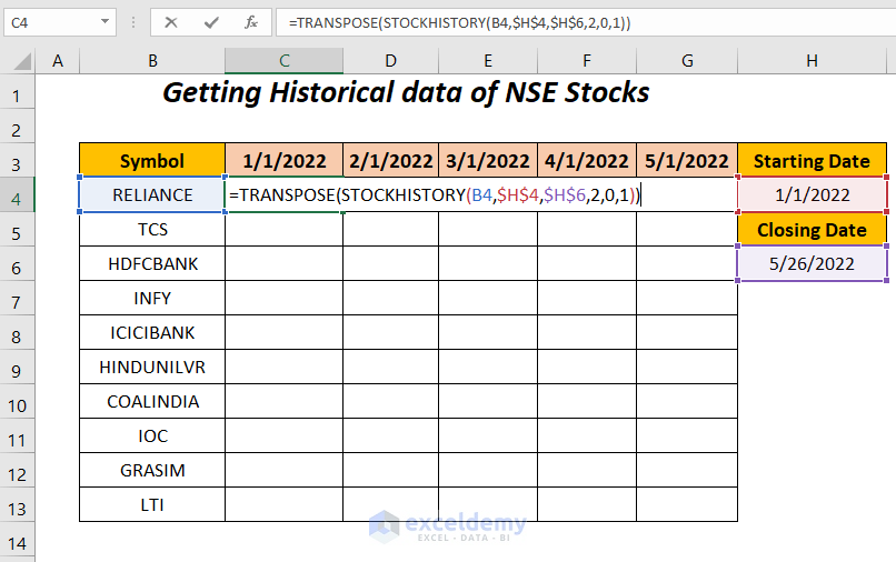
- Press ENTER.
Get the closing stock values from January to May for the RELIANCE company.
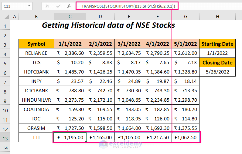
- Drag down the Fill Handle tool.
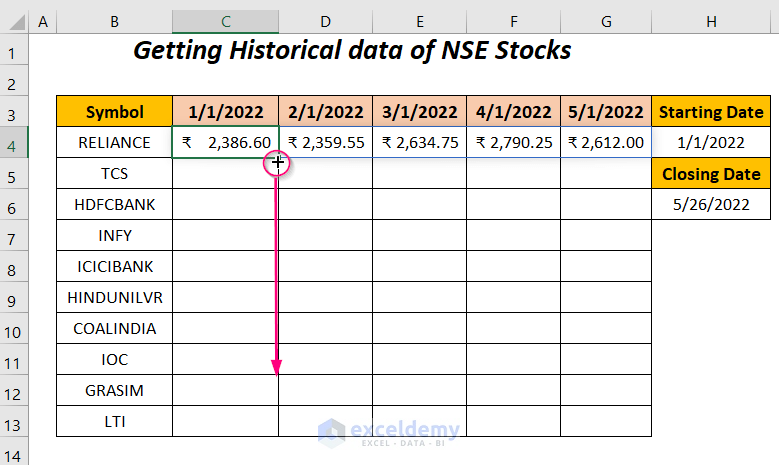
This way, you will get the stock values for the rest of the companies, and the currency symbols here are automatically updated.
Step-04: Exploring Different Properties of STOCKHISTORY Function
In the previous step, we used properties 0 and 1 to gain the dates and the closing stock values for the companies. Use 2 for Opening value, 3 for High value, 4 for Low value, and 5 for the Volume of the amount traded during this period.
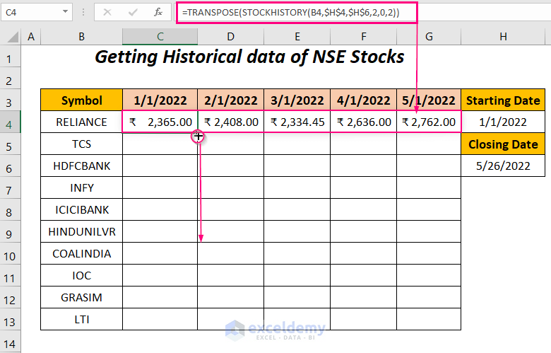
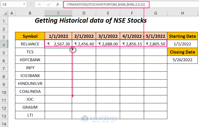
- Use the following formula in cell C4.
=TRANSPOSE(STOCKHISTORY(B4,$H$4,$H$6,2,0,2))Here, the last argument 2 is for Open property.
- Drag the Fill Handle tool.
In this way, you will gather the opening stock values each month for all of the companies.
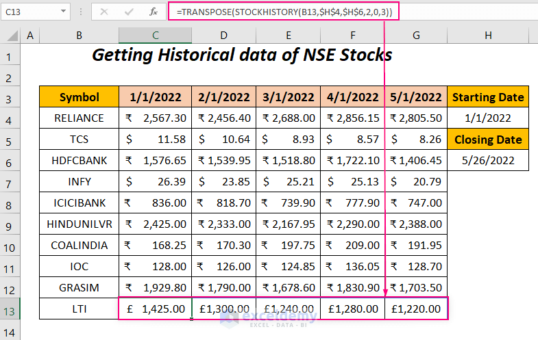
- Apply the following formula in cell C4.
=TRANSPOSE(STOCKHISTORY(B4,$H$4,$H$6,2,0,3))The last argument 3 is for High property.
- Drag down the Fill Handle tool.
We will have high stock values each month for all of the companies.
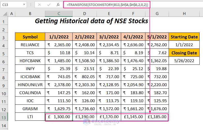
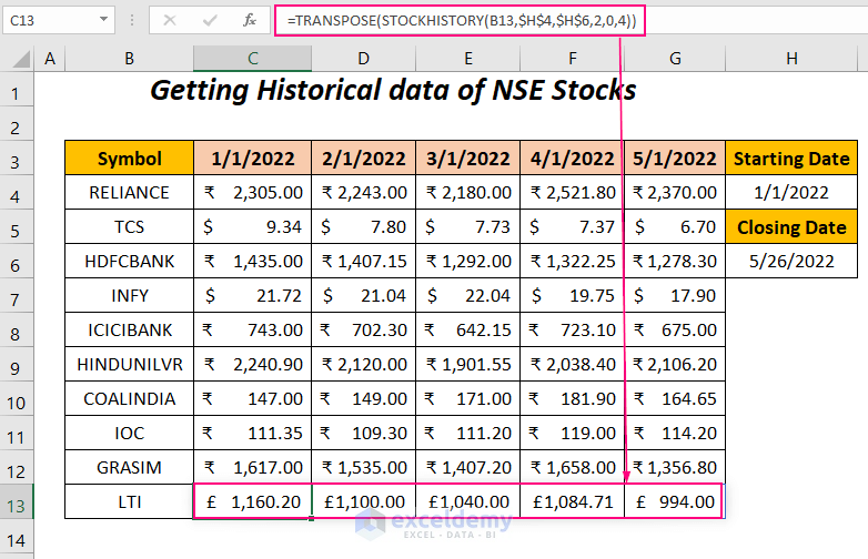
- Type the following formula in cell C4.
=TRANSPOSE(STOCKHISTORY(B4,$H$4,$H$6,2,0,4))The last argument 4 is for Low property.
- Drag the Fill Handle tool.
You will get the companies’ minimum stock values for January to February.
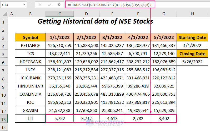
- Apply the following formula in cell C4.
=TRANSPOSE(STOCKHISTORY(B4,$H$4,$H$6,2,0,5))The last argument 5 is for Volume property.
- Drag down the Fill Handle tool.
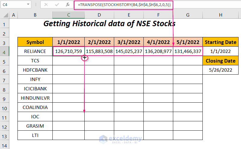
In this way, you will get the volume of the stocks traded each month.
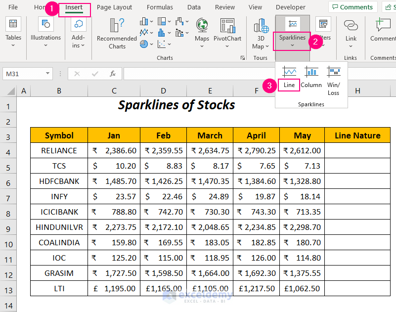
Step-05: Creating Sparklines for Stocks
Add the sparklines of the closing stock values for each company to visualize the characteristics of the change of the stocks over months. To add those lines, we have inserted a new column Line Nature.
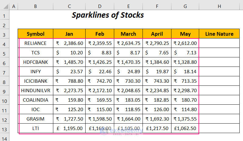
- Go to the Insert Tab >> Sparklines Group >> Line Option.
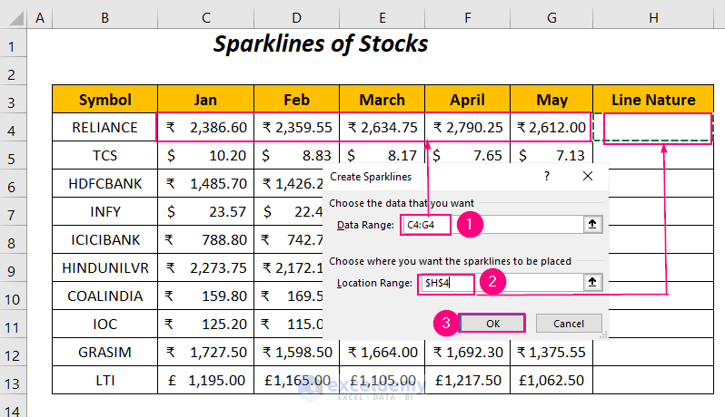
The Create Sparklines dialog box will open up.
- Select the data range of stocks for the RELIANCE company in the Data Range box and $H$4 as the Location Range.
- Press OK.
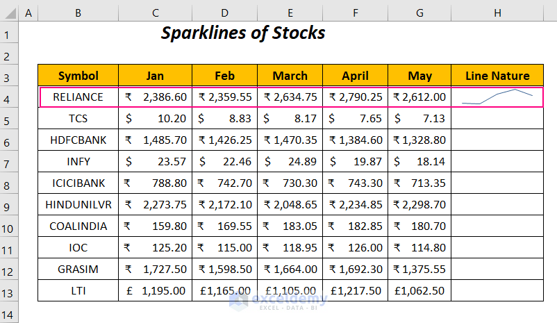
Get the trendline of the stock values nature of the RELIANCE company.
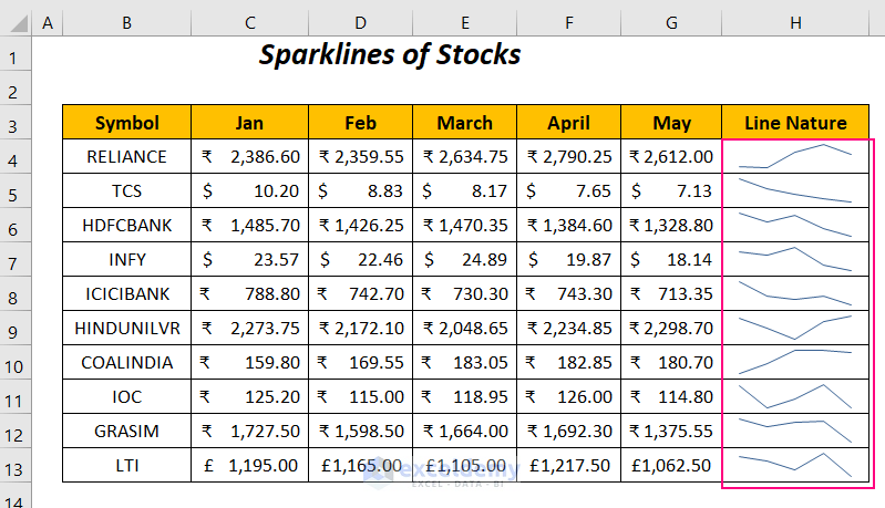
Create the sparklines for other companies to compare the nature of the stock values of these companies.
Method 2 – Using GOOGLEFINANCE Function to Gather Historical Data of NSE Stocks in Google Sheet
If you don’t have the Microsoft Excel 365 version, you can collect the historical data of stocks by using the GOOGLEFINANCE function in Google Sheets.
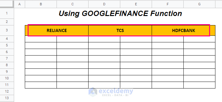
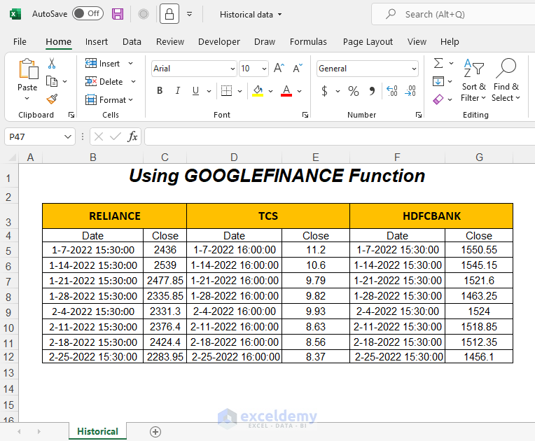
We will demonstrate the process of doing this job for the following 3 companies. We made their names as headers, and each name has 2 columns to gather the dates with the values.
Steps:
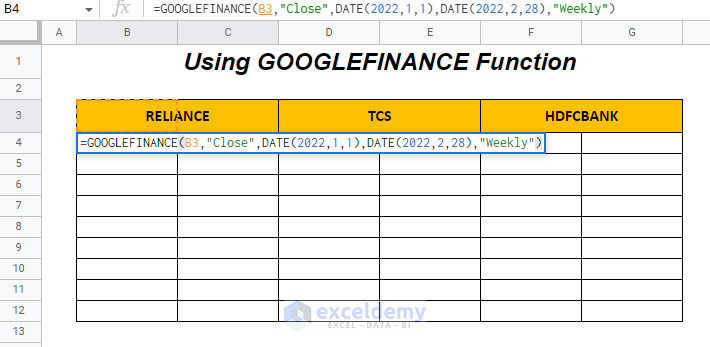
- Use the following formula in cell B3.
=GOOGLEFINANCE(B3,"Close",DATE(2022,1,1),DATE(2022,2,28),"Weekly")B3 is the company’s symbol, “Close” is similar to the property of the above method, DATE(2022,1,1) will return the starting date by using the DATE function, DATE(2022,2,28) will give the end date, and “Weekly” is the interval.
The other properties can be used here; “Open”, “High”, “Low”, “All” etc. We can only get the values for the Daily or Weekly interval.
- Press ENTER.
You will get the weekly closing stock values with corresponding dates and headers as well for the RELIANCE company.

- Use the following 2 formulas for gathering the weekly stock values for the TCS and HDFCBANK companies.
=GOOGLEFINANCE(D3,"Close",DATE(2022,1,1),DATE(2022,2,28),"Weekly")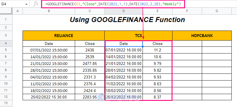
=GOOGLEFINANCE(F3,"Close",DATE(2022,1,1),DATE(2022,2,28),"Weekly")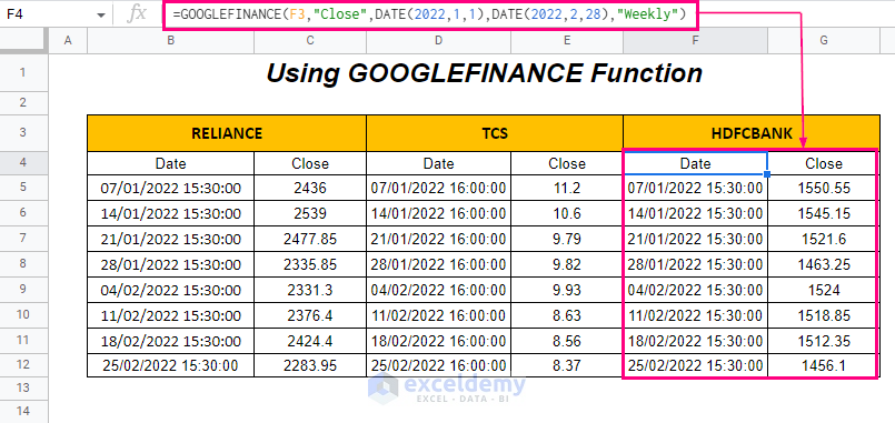
- To save this Google sheet as an Excel file, go to the File Tab >> Download Dropdown >> Microsoft Excel (.xlsx) Option.
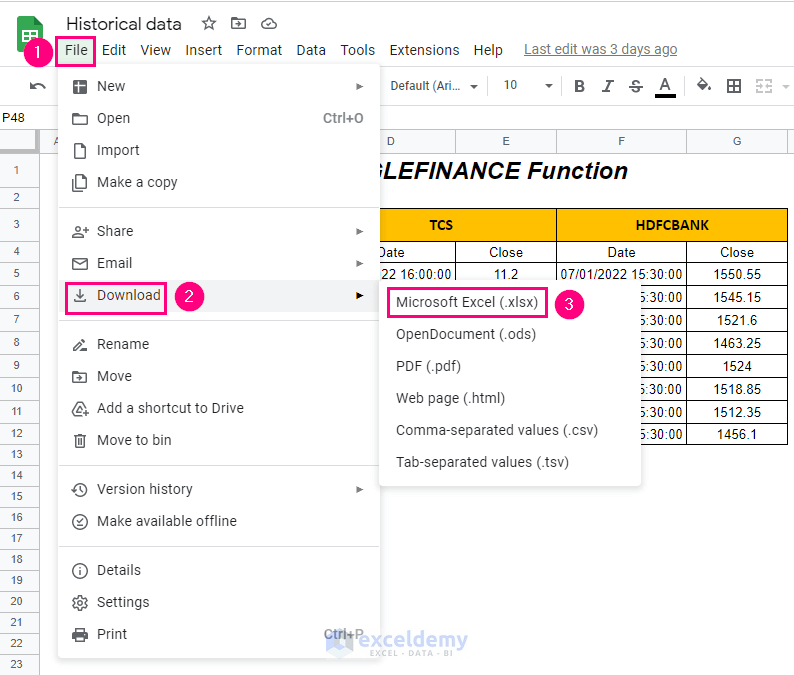
You will get the following sheet in an Excel workbook.
Download Workbook
Related Articles
- How to Add Stock Data Type in Excel (2 Effective Methods)
- How to Get Stock Prices in Excel (3 Easy Methods)
- Stock return analysis using histograms & 4 skewness of histograms
- How to Get Live Stock Prices in Excel (4 Easy Ways)
- How to Get Stock Quotes in Excel (2 Easy Ways)
- GST State Code List in Excel
<< Go Back to Excel Sample Data | Excel Data for Analysis | Learn Excel
Get FREE Advanced Excel Exercises with Solutions!
