How to Make HELOC Payment Calculator Using Principal and Interest in Excel

In this tutorial, I am going to show you the step-by-step procedures to make a HELOC payment calculator using principal and interest in Excel. You can quickly use these steps even in multiple datasets to find the HELOC payment value. Throughout this tutorial, you will also learn some important Excel tools and techniques that will be very useful in any Excel-related task.

What is HELOC?

HELOC stands for Home Equity Line of Credit. It is a special type of loan based on the equity of one’s home mortgage. Also, it is different from other home equity loans like home loans and cash refinances. Below is the formula to calculate HELOC payments.

HELOC Payment =  (CHB × RATE) × ( (1 + RATE)^(12 × RP)) / ( (1 + RATE)^(12 × RP) – 1 )

Where,

CHB = Current HELOC Balance (Principal)

RP= Repayment Periods in Years

RATE= Monthly Interest Rate

Step-by-Step Procedures to Make HELOC Payment Calculator Using Principal and Interest in Excel

We have taken a concise Excel dataset to explain the steps clearly. The dataset has approximately 7 rows and 2 columns. Initially, we formatted all the cells containing dollar values in Accounting format and all the percentage values in % format. For all the datasets, we have 2 unique columns which are Property and Value. Although we may vary the number of columns later on if that is needed.

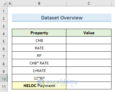
Step 1: Setting Up Data Table

In this first step, we will create the data table to insert the necessary parameters and format them properly.

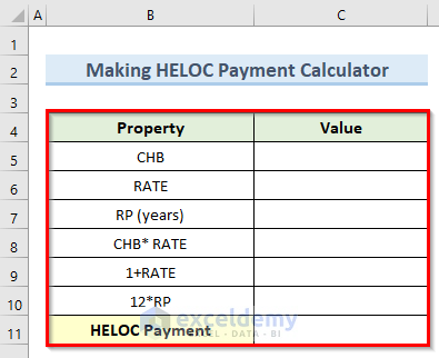
• First, create a data table following the below format and insert the necessary parameters in the left column. Make sure to make the table headers bold.

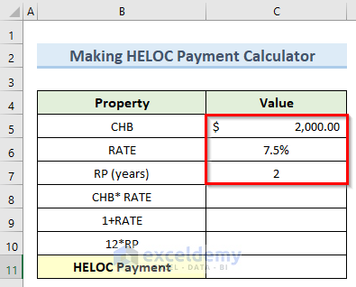
Step 2: Entering Input Values

Now, we have to insert the input values for which we want to calculate our HELOC payments. Let us see how to do that. Alternatively, we can use a HELOC calculator to calculate our payments.

• For this step, type the necessary input values like CHB, RATE, and RP.

Step 3: Finding Monthly Interest-Only Payments and Other Parameters

Here, we will calculate various parameters that we will use inside the final HELOC payment calculation formula. Follow the steps below to do this.

• To begin with, double-click on cell C8 and enter the below formula:

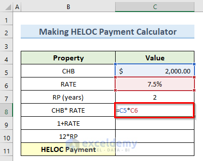
• Next, press the Enter key and you should get the value of CHB times RATE.
• Now, double-click on cell C9 and insert the formula below:

• Next, press the Enter key and consequently, this will find the value of 1+RATE.
• Then, navigate to cell C10 type in the following formula, and press the Enter key again:

Read More: How to Create Annual Loan Payment Calculator in Excel

Step 4: Calculating Final HELOC Payment

Once we have all the input parameters in hand, now we can proceed to the final calculation using the previous values.

• To start this final step, navigate to cell C11 and type in the following formula:

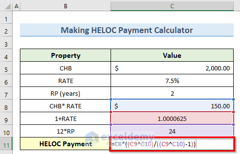
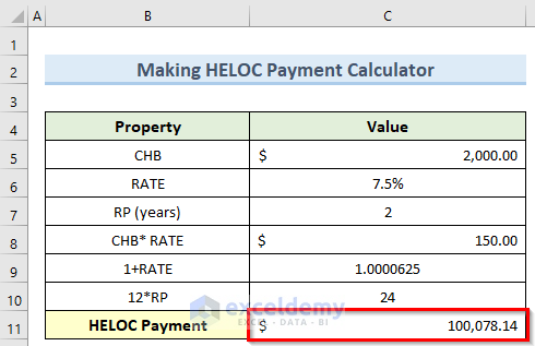
• After that, press the Enter key or click on any blank cell.
• Finally, this will calculate the HELOC Payment value with the help of the necessary parameters.

Download Practice Workbook

You can download the practice workbook from here.

Conclusion

I hope that you were able to apply the methods that I showed in this tutorial on how to make a HELOC payment calculator using principal and interest in Excel. As you can see, there are quite a few steps to achieve this. So follow each of the steps exactly. If you get stuck in any of the steps, I recommend going through them a few times to clear up any confusion. Lastly, If you have any queries, please let me know in the comments.

Related Articles

• Create Progressive Payment Calculator in Excel
• How to Create Snowball Payment Calculator in Excel
• How to Create Line of Credit Payment Calculator in Excel

<< Go Back to Payment Calculator | Finance Template | Excel Templates