How to Make HELOC Payment Calculator in Excel

You can do a wide range of work in Excel worksheets. Excel is a versatile application used in the economic sector. For instance, you can create cash memos or maintain a record of cash flows in Excel. You can also calculate HELOC payment in Excel. In this article, I will show how to make HELOC payment calculator in Excel. I will show four easy steps to make this HELOC calculator in Excel. Hopefully, this will help you to increase your Excel skills.

Introduction to HELOC

Home equity lines of credit are known as HELOC. It’s a unique kind of loan based on the equity in a homeowner’s mortgage. It differs from other home equity loans, such as mortgages and cash refinances, as well. I will show the calculation method for HELOC payments below.

HELOC Payment = (CHB × RATE) × ( (1 + RATE)^(12 × RP)) / ( (1 + RATE)^(12 × RP) – 1 )

Where,

CHB = Current HELOC Balance (Principal)

RP= Repayment Periods in Years

RATE= Monthly Interest Rate

Step-by-Step Procedures to Make HELOC Payment Calculator in Excel

Here, I will consider a dataset about the Payment Details of ABC Traders. The dataset has two columns, B and C called Property and Value. The dataset ranged ranges from B4 to C11. The Value column is blank here. I will input the required values step by step and will complete all the procedures shown below. The process is not so complex. I have added the necessary images with the steps for your convenience.

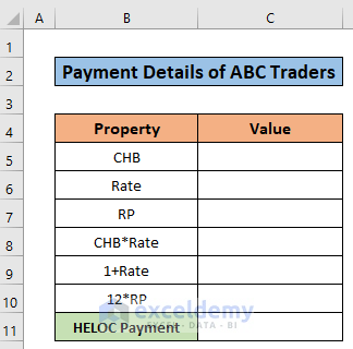
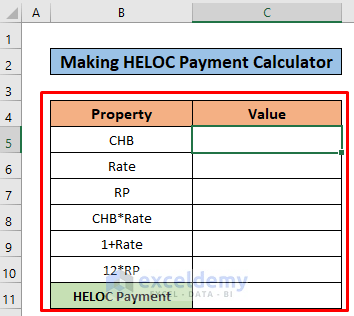
Step 1: Making the Dataset

This is the first step of this article. Here I will make the dataset. Follow the steps given below and make a dataset similar to mine.

I have selected 8 rows and 2 columns for the dataset.
The two columns B and C are called Property and Value.

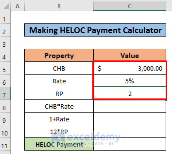
Step 2: Entering the Input Values

Now, I will describe the second step of this procedure, I will Input the required values here. Follow the steps and images to make a HELOC payment calculator in Excel.

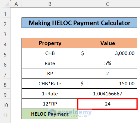
First Enter the value of 3000 dollars as CHB in the C5 cell.
Then, input the Rate value of 5% in the C6 cell.
After that, enter the RP value as 2 in the C7 cell.

Step 3: Calculating Monthly Interests with Other Parameters

This is the most important step of this article. I will calculate different important parameters of making a HELOC payment calculator. These parameters have an important influence on the calculation of HELOC payments. So follow the steps carefully. Moreover, I hope this will increase your Excel skill.

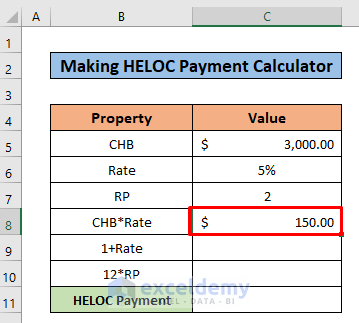
First, select the C8 cell.
Additionally, write down the following formula in the C8 cell.

=C5*C6

Then, press the enter button.

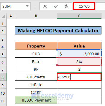
Consequently, you will find the result of 150 dollars in the C8 cell.

After that, select the C9 cell.
Write down the following formula in the selected cell.

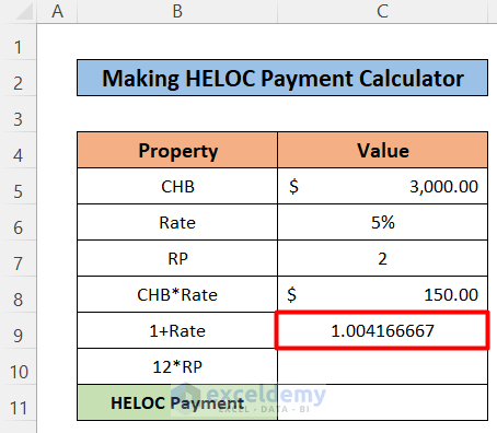
=1+((C6)/12)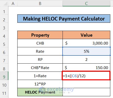

After pressing Enter, you will find the result like the picture given below.

Now, select the C10 cell.
After that, copy the following formula in the selected cell.

=12*C7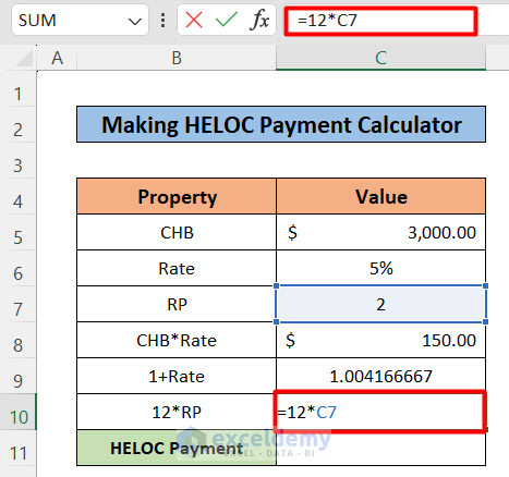

After pressing enter, you will find the result like the picture given below.

Step 4: Calculating Final HELOC

This is the last step of this article. At the last point of this article, you will calculate the final HELOC for the ABC Traders. Follow the simple steps mentioned below.

Select the C11 cell first.
After that, copy the following formula in the C11 cell.

=C5*C6*((C9^C10)/((C9^C10)-1))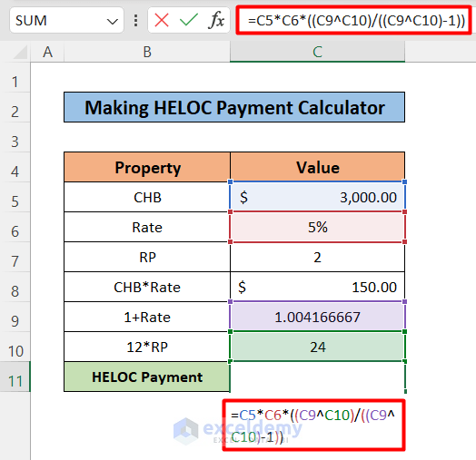

Meanwhile, press the enter button.
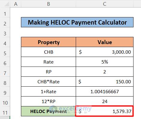
As a consequence, you will get the final HELOC payment in cell C11.

Things to Remember

Be careful about the parameters you have used in the whole process as they have an impact on the calculation of HELOC Payment.

Download Practice Workbook

Please download the workbook to practice yourself.

HELOC Payment Calculator.xlsx

Conclusion

In this article, I have tried to explain how to make a HELOC payment calculator in Excel. I hope you have learned something new from this article. Now, extend your skill by following the steps of these methods. . However, I hope you have enjoyed the whole tutorial. Moreover, If you have any queries, feel free to ask me in the comment section. Don’t forget to give us your feedback.

<< Go Back to Payment Calculator | Finance Template | Excel Templates

Get FREE Advanced Excel Exercises with Solutions!

4 Comments

Tom Jul 25, 2023 at 9:08 PM

What is the little up arrow carrot between c9 and c10 in the resultant formula of the heloc
Alif Bin Hussain Jul 26, 2023 at 10:24 AM

Hello Tom,

The upward arrow between C9 and C10 in the formula indicates the exponent operation of mathematics. In the formula, C9 raised to the power of C10 is written as C9^C10. A simple example would be “Two Squared” which is written as 2^2 = 4, where 2 is raised to the power of 2, resulting in 4.
test Sep 13, 2023 at 10:40 PM

Thank you, but hard to see how this can be correct. In your example, you borrow $3000, and if you have to pay back in 2 years at 5%, your total payment will be $150,000? That does not sound right.
- Reply
  Tanjim Reza Sep 19, 2023 at 5:51 PM
  
  Hello, Test. Thank you for this beautiful feedback.
  
  Yes, you are right. This doesn’t seem right. We found the error as we were dividing the interest rate by 100 even though it was already in Percentage format. As a result, our answer got multiplied by 100 later. That is, when calculating the 1+Rate value, we had to divide cell C6 by only 12, not 100 and 12 both.
  We have fixed the error now. You can go through the corrected article again and download our corrected workbook too.
  However, this article is written on the basis of compound interest. You can also use the simple interest formula here to find your simple HELOC Payment.
  
  With Regards,
  Md. Tanjim Reza Tanim