How to Interact with a Target Cell Using Excel VBA (9 Examples)

Understanding the Target Cell Property

When you want to interact with a cell in a worksheet using an event, you can utilize the Target property of Excel. These events are triggered when you perform actions like changing the value of a cell or selecting a range. One commonly used event is the Worksheet Change event, which fires whenever a cell is modified in the worksheet. The Target cell refers to the cell that was changed by the user, and we can use it to perform specific tasks such as formatting or displaying a message box based on the user’s input.

Enabling the VBA Environment

Before we dive into the examples, make sure you have the VBA environment set up in Excel. Here are two ways to access it:

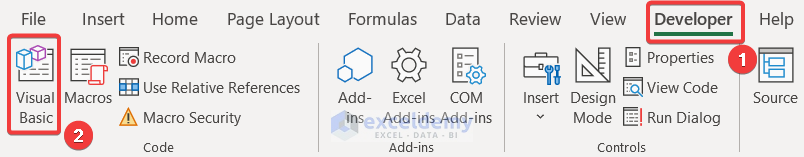
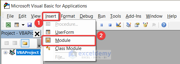
• Using the Module Window
  • Open the Developer tab (if you don’t see it, enable it).
  • Select the Visual Basic command.

• • The Visual Basic window will open, and you can insert a Module from the Insert menu to enter your VBA code.

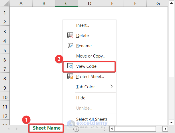
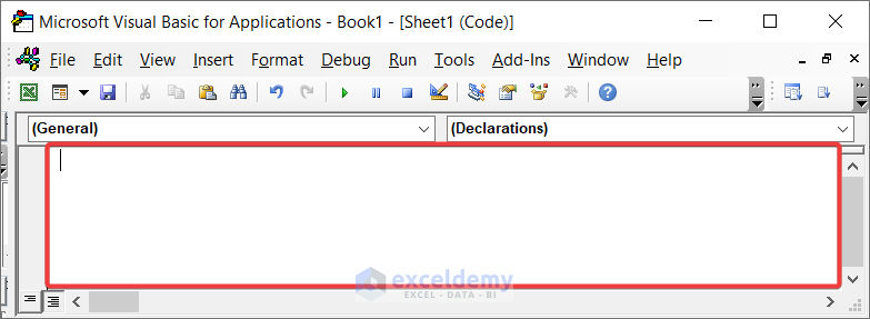
• Utilizing the Sheet Code Window
  • Right-click on the worksheet name and choose View Code.

• • Enter your code in the window that appears.

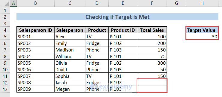
Example 1 – Checking If the Target Cell Contains a Certain Value

Suppose we have a dataset called Sales Data, and we want to check if the Total Sales values in cells F12 and F13 exceed a target value of 30.

We can achieve this using the following VBA code:

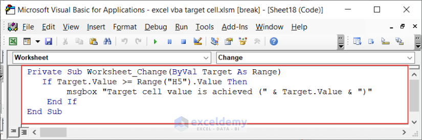
Private Sub Worksheet_Change(ByVal Target As Range)
If Target.Value >= Range("H5").Value Then
msgbox "Target cell value is achieved (" & Target.Value & ")"
End If
End Sub

Read More: How to Use Target Value in Excel VBA

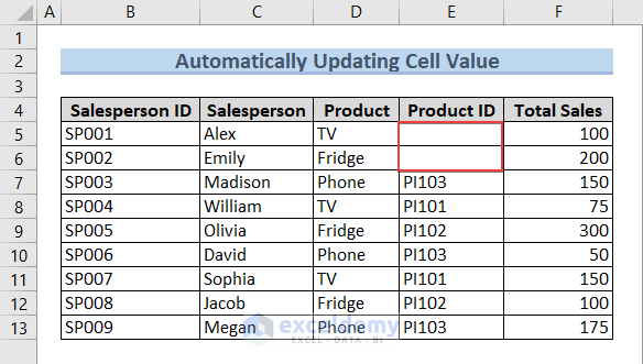
Example 2 – Updating the Target Cell Value

In this scenario, we’ll enter Product IDs into cells starting from E5. Note that the Product IDs contain the prefix PI. Our dataset looks like this:

To automatically insert the prefix in the Product ID data using VBA, we’ll create the following macro:

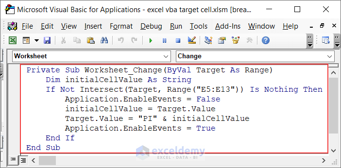
Private Sub Worksheet_Change(ByVal Target As Range)
Dim initialCellValue As String
If Not Intersect(Target, Range("E5:E13")) Is Nothing Then
Application.EnableEvents = False
initialCellValue = Target.Value
Target.Value = "PI" & initialCellValue
Application.EnableEvents = True
End If
End Sub

When we insert a Product ID value in cells E5:E13, the prefix “PI” is automatically added.

Example 3 – Setting the Font Style to Bold for the Target Cell

In this case, we want to bold a specific Salesperson ID, which is SP009. Our dataset looks like this:

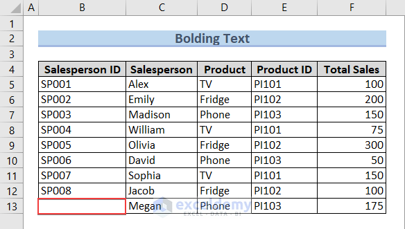
To achieve this using VBA, we’ll enter the following code:

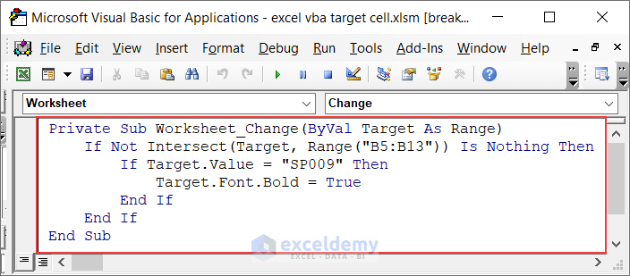
Private Sub Worksheet_Change(ByVal Target As Range)
If Not Intersect(Target, Range("B5:B13")) Is Nothing Then
If Target.Value = "SP009" Then
Target.Font.Bold = True
End If
End If
End Sub

When we enter SP009 in the specified range, the font becomes bold.

Example 4 – Changing the Font Color of the Target Cell

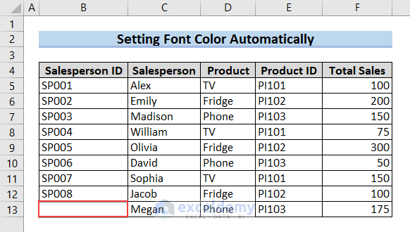
In this example, we’ll change the font color from the default to blue when a change occurs in the specified range (B5:B13). Our dataset looks like this:

To set the font color of the target cell using VBA, we’ll enter the following macro:

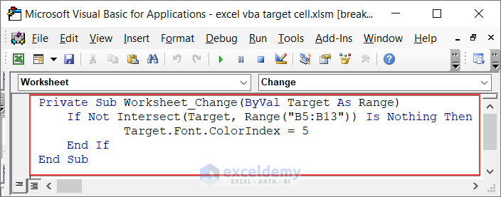
Private Sub Worksheet_Change(ByVal Target As Range)
If Not Intersect(Target, Range("B5:B13")) Is Nothing Then
Target.Font.ColorIndex = 5
End If
End Sub

Now, any changes in the specified range will update the font color accordingly.

Example 5 – Uppercasing the Target Cell

In this example, we’ll convert the input of cells within our specified range (B5:B13) to uppercase. Our dataset looks like this:

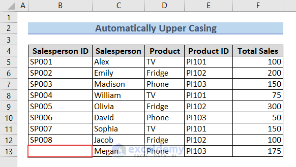
The data under the Salesperson ID column must be in uppercase. To achieve this, we’ll use VBA. Here’s the code snippet:

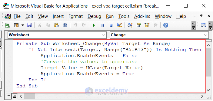
Private Sub Worksheet_Change(ByVal Target As Range)
If Not Intersect(Target, Range("B5:B13")) Is Nothing Then
Application.EnableEvents = False
'Convert the values to uppercase
Target.Value = UCase(Target.Value)
Application.EnableEvents = True
End If
End Sub

Any changes in the specified range will automatically convert the cell values to uppercase.

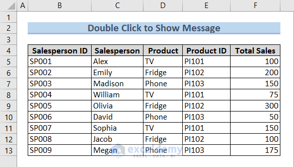
Example 6 – Enabling a Double Click Event with the Target Cells

In this case, we’ll demonstrate how to enable a double-click event with the target cell. We’ll specify a range of cells in the worksheet. Then, if we double-click on any specific cell within that range, a message will display the cell value.

Our dataset looks like this:

To achieve this using VBA, we’ll enter the following code:

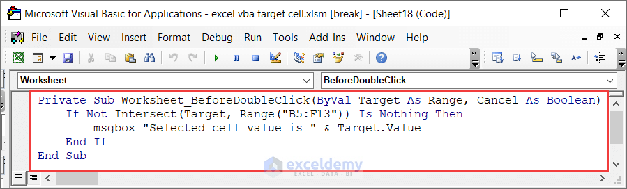
Private Sub Worksheet_BeforeDoubleClick(ByVal Target As Range, Cancel As Boolean)
If Not Intersect(Target, Range("B5:F13")) Is Nothing Then
msgbox "Selected cell value is " & Target.Value
End If
End Sub

When we double-click on any cell within the specified range (e.g., F7), the value of that cell will be displayed.

Read More: How to Use Excel VBA Target Range

Example 7 – Automatically Updating Columns Based on Changes in the Target Cell

In Excel VBA, we can leverage the Target cell property to automatically update columns when changes occur. For instance, whenever we modify data in a worksheet, we might want to propagate those changes to another worksheet. Let’s walk through an example.

Scenario

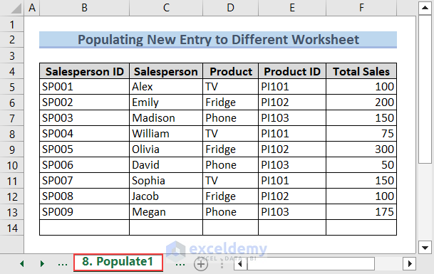
1. We have a worksheet named Sheet19 where we’ll make changes to cell values.
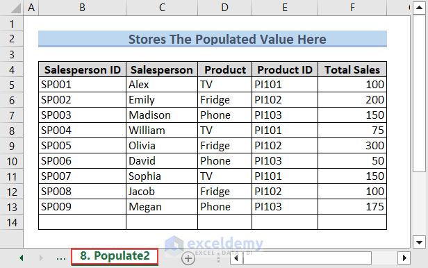
2. Whenever a change occurs in Sheet19, we want to populate the modified cell values in a different worksheet called Sheet21.

VBA Code

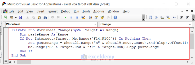
Private Sub Worksheet_Change(ByVal Target As Range)
Dim pasteRange As Range
If Not Intersect(Target, Me.Range("F14:F100")) Is Nothing Then
Set pasteRange = Sheet21.Range("B" & Sheet19.Rows.Count).End(xlUp).Offset(1)
Me.Range("B" & Target.Row & ":F" & Target.Row).Copy pasteRange
End If
End Sub

Any changes in the Sheet 19 worksheet will automatically update the corresponding columns in the Sheet 21 worksheet.

Read More: Excel VBA: How to Use Target Row

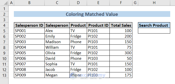
Example 8 – Coloring Matched Values

Suppose we have a dataset, and we want to search for specific products. Whenever a product in cell H5 matches an entry in the dataset (column D), we want to highlight that product in column D. Let’s achieve this using VBA.

Dataset

VBA Code

The following image contains the VBA code to do so.

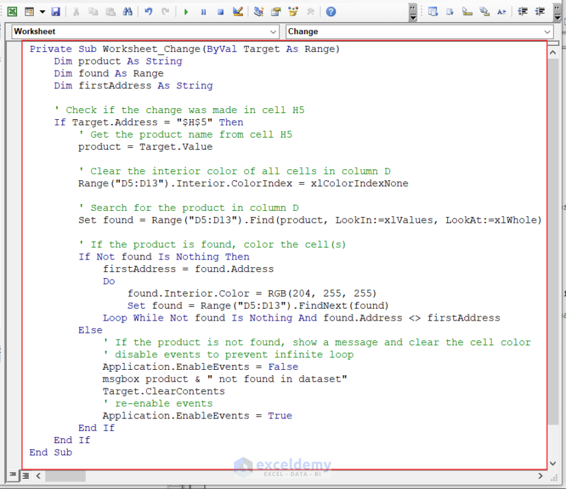
Private Sub Worksheet_Change(ByVal Target As Range)
Dim product As String
Dim found As Range
Dim firstAddress As String
' Check if the change was made in cell H5
If Target.Address = "$H$5" Then
' Get the product name from cell H5
product = Target.Value
' Clear the interior color of all cells in column D
Range("D5:D13").Interior.ColorIndex = xlColorIndexNone
' Search for the product in column D
Set found = Range("D5:D13").Find(product, LookIn:=xlValues, LookAt:=xlWhole)
' If the product is found, color the cell(s)
If Not found Is Nothing Then
firstAddress = found.Address
Do
found.Interior.Color = RGB(204, 255, 255)
Set found = Range("D5:D13").FindNext(found)
Loop While Not found Is Nothing And found.Address <> firstAddress
Else
' If the product is not found, show a message and clear the cell color
' disable events to prevent infinite loop
Application.EnableEvents = False
msgbox product & " not found in dataset"
Target.ClearContents
' re-enable events
Application.EnableEvents = True
End If
End If
End Sub

If we search for any product in the dataset, for example, TV, then we need to enter TV in cell H5.

Example 9 – Coloring Cells Based on Conditions

In Excel VBA, we can use the Target cell property to dynamically color cells based on specific conditions. Let’s explore two scenarios: coloring cells containing integer values and coloring cells containing string values.

9.1 Color Cells Containing Integer Values Based on Condition

Suppose we want to color the Total Sales values based on specific criteria. Initially, our dataset looks like this:

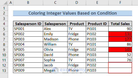
We’ll automatically color the cells red if their values fall between 100 and 200. Let’s achieve this using VBA. Here’s the code snippet:

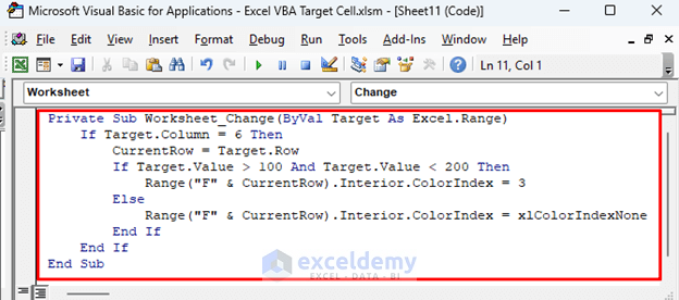
Private Sub Worksheet_Change(ByVal Target As Excel.Range)
    If Target.Column = 6 Then
        CurrentRow = Target.Row
        If Target.Value > 100 And Target.Value < 200 Then
            Range("F" & CurrentRow).Interior.ColorIndex = 3
        Else
            Range("F" & CurrentRow).Interior.ColorIndex = xlColorIndexNone
        End If
    End If
End Sub

If we enter the Total Sales values in those cells, the cells containing values between 100 and 200 will be colored red automatically.

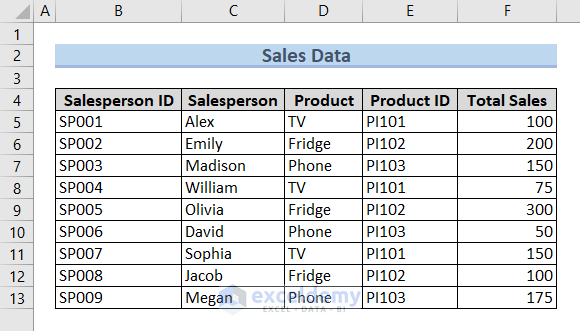
9.2 Color Cells Containing String Values Based on Condition

Now let’s consider coloring cells based on specific string values. Suppose we want to highlight products in the Product column with different colors. We’ll use separate colors for TV, Phone, and Fridge. Our dataset looks like this:

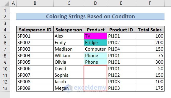
To achieve this using VBA, we’ll enter the following code:

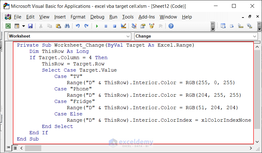
Private Sub Worksheet_Change(ByVal Target As Excel.Range)
Dim ThisRow As Long
If Target.Column = 4 Then
ThisRow = Target.Row
Select Case Target.Value
Case "TV"
Range("D" & ThisRow).Interior.Color = RGB(255, 0, 255)
Case "Phone"
Range("D" & ThisRow).Interior.Color = RGB(204, 255, 255)
Case "Fridge"
Range("D" & ThisRow).Interior.Color = RGB(51, 204, 204)
Case Else
Range("D" & ThisRow).Interior.ColorIndex = xlColorIndexNone ' no color
End Select
End If
End Sub

If we enter the Product in the cells in column D, the cells will color accordingly.

How to Write to Multiple Cells Using the Target.Address Method in Excel VBA

Sometimes, we need to perform tasks based on specific conditions in Excel. For instance, if we want to calculate the total sales of the first two salespeople, we can achieve this using the Target.Address property in VBA. Let’s explore how to do this.

Scenario

Suppose we have a dataset with Total Sales values, and we want to compute the non-zero sum of the Total Sales for the first two salespeople.

VBA Code Example

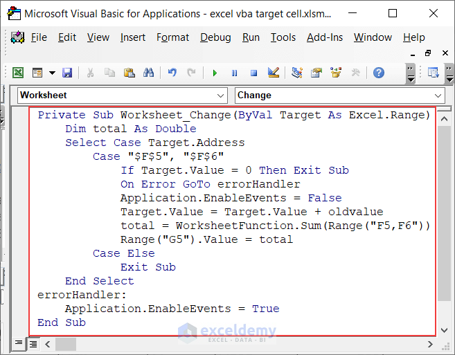
Private Sub Worksheet_Change(ByVal Target As Excel.Range)
Dim total As Double
Select Case Target.Address
Case "$F$5", "$F$6"
If Target.Value = 0 Then Exit Sub
On Error GoTo errorHandler
Application.EnableEvents = False
Target.Value = Target.Value + oldvalue
total = WorksheetFunction.Sum(Range("F5,F6"))
Range("G5").Value = total
Case Else
Exit Sub
End Select
errorHandler:
Application.EnableEvents = True
End Sub

Whenever you modify the Total Sales values in cells F5 or F6, the Target.Address method calculates the non-zero sum for the first two salespeople.

Download Practice Workbook

You can download the practice workbook from here: