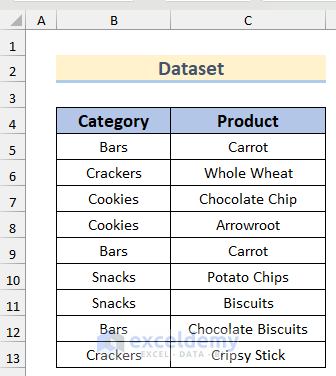
We have entries of certain Categories and Products in a dataset. We’ll check if a cell contains text and then return a value in Excel.
Method 1 – Use the IF Function to Check If Cell Contains Text, Then Return a Value
The syntax of the IF function is:
=IF (logical_test,[value_if_true],[value_if_false])Steps:
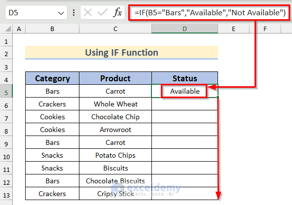
- Select Cell D5 and insert the following formula.
=IF(B5="Bars","Available","Not Available")- Press Enter and drag the Fill Handle down to copy the formula for the rest of the cells.
- Available or Not Available values will appear throughout the range.
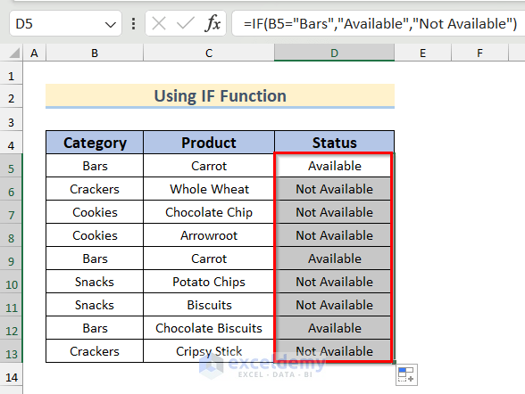
Here, the logical_test is to match Bars text in cell B5; if the test is TRUE it results in Available, otherwise Not Available.
Method 2 – Use the IF and ISTEXT Functions to Check If Cell Contains Text, Then Return Value
Steps:
- Insert the following formula in Cell D5 and press Enter.
=IF(ISTEXT(B5),B5,"")- Drag down the Fill Handle tool to AutoFill the formula for the rest of the cells.
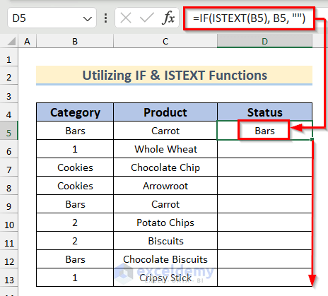
- The formula will return only the text values.
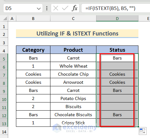
How Does the Formula Work?
- We used the ISTEXT function to check if Cell B5 contains text.
- We used the IF function to return the value of Cell B5 if the result of the ISTEXT function is TRUE. Otherwise, we return a Blank.
Method 3 – Apply ISNUMBER and SEARCH Functions to Find If a Cell Contains Text
Steps:
- Click on Cell D5 and insert the following formula.
=ISNUMBER(SEARCH("Bars",$B$5:$B$13))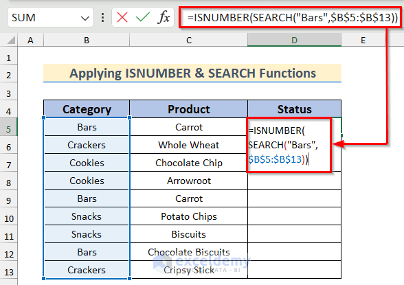
- Press Enter.
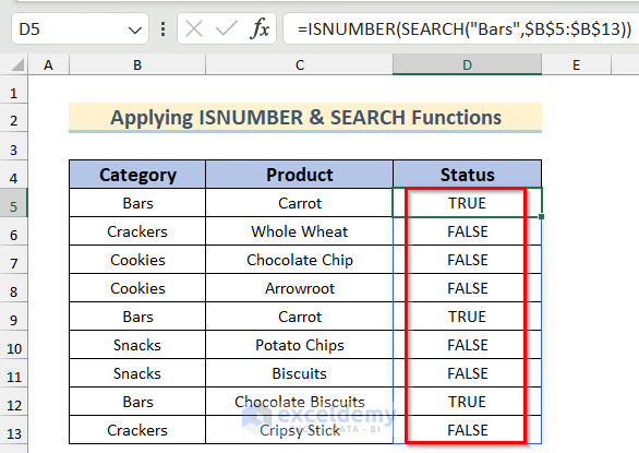
The SEARCH function matches the text “Bars” in an absolute range and then returns True or False depending on the match.
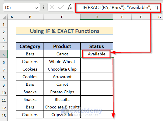
Method 4 – Check If Cell Contains Text, Then Return Value in Excel Using IF and EXACT Functions
This formula works for a case-sensitive match.
Steps:
- SWelect Cell D5 and paste the following formula.
=IF(EXACT(B5,"Bars"),"Available","")- Hit Enter.
- Drag the Fill Handle to copy the formula.
- Here are the results.
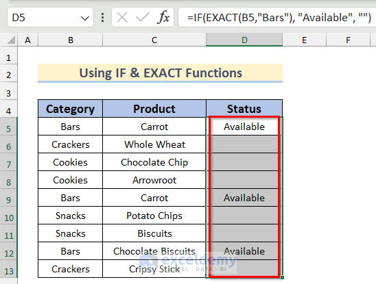
The EXACT function matches the exact text “Bars” in cell B5 then returns the value “Available” otherwise BLANK the cell depending on an exact match.
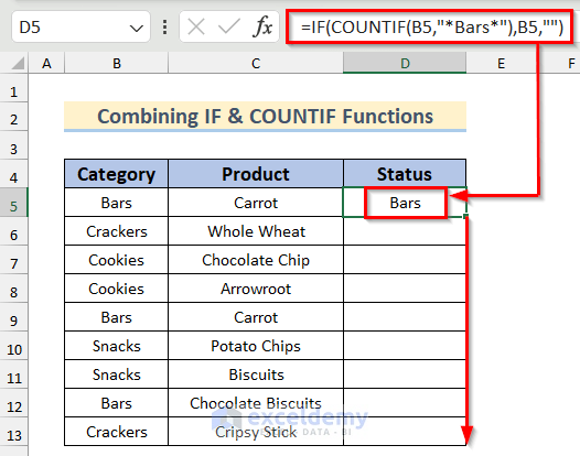
Method 5 – Combine IF and COUNTIF Functions to Check If a Cell Contains Text
Steps:
- Insert the following formula in Cell D5 and press Enter.
=IF(COUNTIF(B5,"*Bars*"),B5,"")- Drag down the Fill Handle tool to AutoFill the formula for the rest of the cells.
- Matching cells will show the same values as the range.
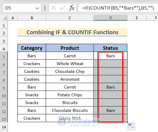
In the formula, the COUNTIF function matches the criteria “*Bars*” (the formula automatically puts * both sides of the criteria) in range (cell B5). Then it returns the value in B5 otherwise keeps the cell Blank.
Method 6 – Use INDEX and MATCH Functions to Find If Cell Contains Text, Then Return a Value in Excel
Steps:
- Insert the following formula in Cell C15.
=INDEX(C5:C13,MATCH("Bars",B5:B13,0))- Press Enter if you’re using Excel 365, or press Ctrl + Shift + Enter.
- The matched text for Bars will appear.
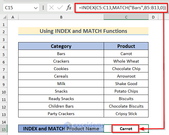
The INDEX function looks for the exact match text “Bars” from the range B5:B13 in the range C5:C13.
Method 7 – Apply the VLOOKUP Function to Check If a Cell Contains Text in Excel
Steps:
- Insert the lookup text (Bars) in any cell (B16).
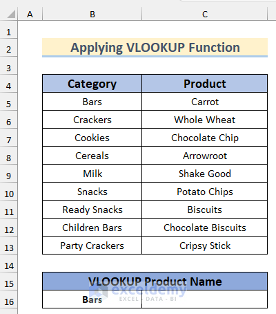
- Select Cell C16 and insert the following formula.
=VLOOKUP(B16,B5:C13,2,FALSE)- Press Enter and the matched value will appear.
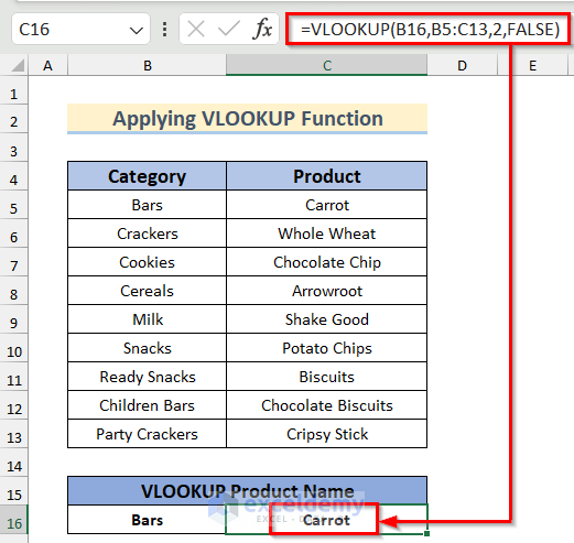
Here “Bars” is the text in B3 that has to match within a range B7:C15 to a value in column 2. FALSE declares we want an exact match.
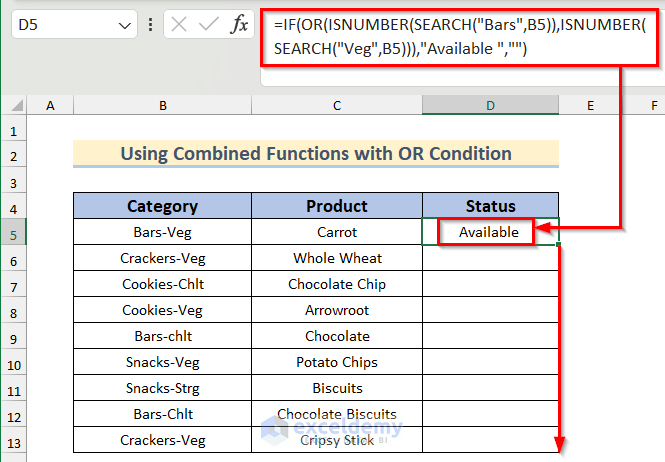
Method 8 – Use Combined Functions to Check if a Cell Contains Text with OR Conditions
Steps:
- Insert the following formula in Cell D5 and press Enter.
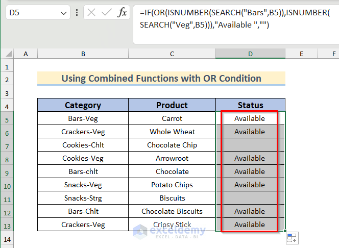
=IF(OR(ISNUMBER(SEARCH("Bars",B5)),ISNUMBER(SEARCH("Veg",B5))),"Available","")- Drag down the Fill Handle tool to AutoFill the formula for the rest of the cells.
- Here’s the result.
How Does the Formula Work?
- We used the SEARCH function to find cell range Bars in Cell B5.
- We used the ISNUMBER function to check if the result of the SEARCH function is a number.
- We searched for Veg in Cell B5 using these two functions.
- We used the OR function to check if any of these two texts (Bars or Veg) is present in Cell B5.
- We used the IF function to return Available if True or leave the cell blank otherwise.
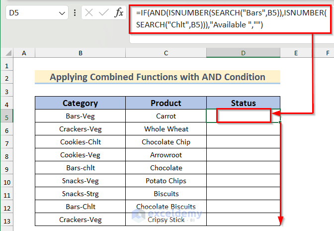
Method 9 – Check If a Cell Contains Text with an AND Condition by Applying Combined Functions
Steps:
- Select Cell D5 and insert the following formula.
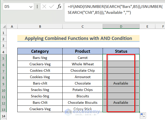
=IF(AND(ISNUMBER(SEARCH("Bars",B5)),ISNUMBER(SEARCH("Chlt",B5))),"Available ","")- Press Enter. If both of the text strings exist in cell B5, the formula returns “Available” as a value. Otherwise, the cell remain BLANK.
- Drag the Fill Handle to copy the formula for the rest of the cells.
- Here are the results.
How Does the Formula Work?
- We used the SEARCH and ISNUMBER functions like Method 8.
- We used the AND function to check if these two texts (Bars and Veg) are present in Cell B5.
- We used IF function to return Available if True, otherwise Blank.
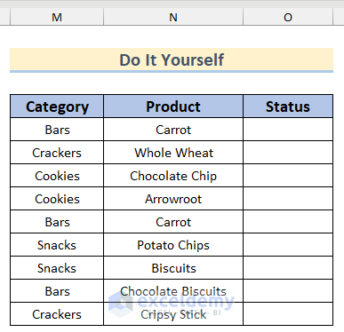
Practice Section
We attached a practice dataset that you can use to test these methods.
Download the Practice Workbook
<< Go Back to Text | If Cell Contains | Formula List | Learn Excel
Get FREE Advanced Excel Exercises with Solutions!

If some idiot changes the dollar value by putting a text character in it, how do I get just the value? Not of these methods seem to help.
Cell = ‘50.50 I want to get the value Cell 2 = 50.50 Where is this covered?
Greetings Dr. Linda Vandergriff,
Go through the following methods to get rid of the inconvenience. Make sure the value cells are in the Currency or Accounting Number Format.
1. Manually delete the preceding Apostrophes. Or
2. Use a formula to auto remove the Apostrophes as shown in the image.
=NUMBERVALUE(SUBSTITUTE(B2,"'",""))Feel free to comment if you have further inquiries. We are here to help.
Regards
Maruf Islam (Exceldemy Team)
HI, I want to pull text from multiple sheets and ignore some specific text as blank or space. How to do it?
Example .
If sheet 1 has John in B2 and sheet2 has Jacob in B2 and i want an output in sheet3, where if sheet 2 has Jacob then ignore or blank.
=Sheet1!B2&” “&Sheet2!B2
Hi Mohammed Shahid,
You can pull text from multiple sheets and ignore blank or space by using the TRIM function. This function will help you to remove space automatically.
To solve your problem, use the following formula in Cell B2 of Sheet 3 in your Excel worksheet.
=TRIM(Sheet1!B2&" "&Sheet2!B2)Hope this will solve your problem. Feel free to comment if you have further inquiries.
Regards,
Arin Islam.
Hello, is it possible to somehow combine the EXACT and IF & ISTEXT Functions to return the text value of two cells in different columns instead of TRUE/FALSE? I am trying to match answers to two slightly different questions in a survey which have the same list of potential answers.
Hello JAMES
Thanks for reaching out and sharing your queries. To return the text value of two cells in different columns if they match, you can combine the EXACT, IF and ISTEXT functions.
Excel Formula:
=IF(AND(ISTEXT(A2), ISTEXT(B2), EXACT(A2, B2)), A2:B2, "No Match")So, in simpler terms, the formula checks if both cells A2 and B2 contain text and if the text in both cells is the same. If they are, it returns the values from cells A2 and B2 together. If not, it returns “No Match”.
OUTPUT:
Hopefully, the idea will help you; good luck.
Regards
Lutfor Rahman Shimanto
ExcelDemy
Hi, is it possible to have a column return a value based on multiple values in another column?
Ex:
Column A’s cells each have one color: Red, Orange, Yellow, Green, Blue, Purple
Column B should return a value based on if A is one of several of those colors.
Is it possible to do this with two formulas based on the output value, or would I need to make six formulas (one for each input value)
Ideally for two I would want formulas:
If the cell in A has either Red, Orange, or Yellow then column B in that row will return “Warm”
If the cell in A has either Green, Blue, or Purple then column B in that row will return “Cool”
Hello Rat,
It is possible to return a single value based on muliple values of another column. You can do it by using combination of the nested IF and OR functions without needing six separate formulas.
Use the following formula and drag the fill handle down to apply the formula to the rest of the cells in Column B.
=IF(OR(A2=”Red”, A2=”Orange”, A2=”Yellow”), “Warm”, IF(OR(A2=”Green”, A2=”Blue”, A2=”Purple”), “Cool”, “”))
The formula uses OR to check if the color in Column A matches any “Warm” colors (Red, Orange, Yellow) and returns “Warm”; if it matches any “Cool” colors (Green, Blue, Purple), it returns “Cool”. If none of these are true, it returns an empty value.
Regards
ExcelDemy
I have a string of text in column T on tab 1, but need to determine if it contains a smaller string of text from a table on tab 2. Then I need column U on tab 1 to return the text from column B on tab 2. What combo of formulas will work? I’ve tried vlookup, search, countif… and others, but I cannot get the correct combination.
Hello Amy,
You can try using a combination of SEARCH and INDEX-MATCH.
In cell U2 on Tab 1, try the following formula:
=IFERROR(INDEX(‘Tab 2’!B:B, MATCH(TRUE, ISNUMBER(SEARCH(‘Tab 2’!A:A, T2)), 0)), “”)
1. SEARCH(‘Tab 2’!A:A, T2) checks if any value from column A on Tab 2 is found in the text in column T on Tab 1.
2. INDEX(‘Tab 2’!B:B, …) returns the corresponding value from column B on Tab 2.
3. IFERROR handles cases where no match is found.
This should return the desired result in column U of Tab 1.
Regards
ExcelDemy