Method 1 – Using Excel Power Query Editor to Combine 2 Columns
Steps:
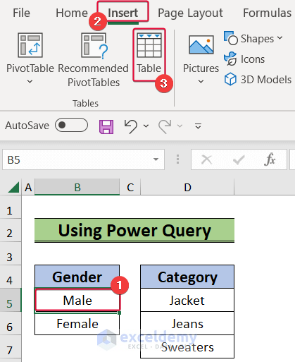
- Select cell B5 in the Gender column.
- Go to the Insert tab.
- Select Table.
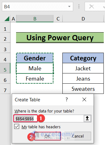
- A prompt will open on the screen.
- Select B5:B6 as the table range and click.
- The range will be converted into a table.
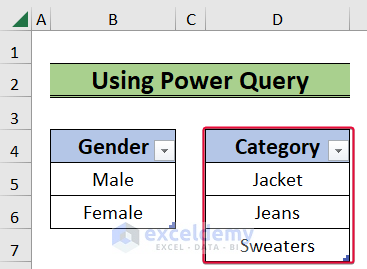
- Repeat the process for the Category column and turn it into a table.
- Select cell B5 and go to the Data tab.
- From the Data tab, select From Table/Range.
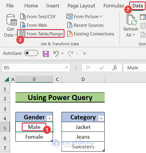
- The column will open in the Power Query window.
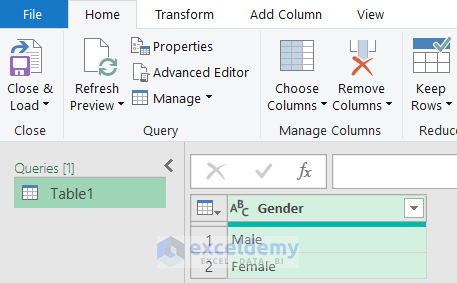
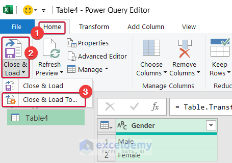
- In the Power Query window, go to the Home tab.
- Select Close & Load To from the Close & Load option.
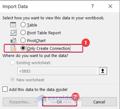
- A prompt will open on the screen.
- Choose the Only Create Connection option.
- Click OK.
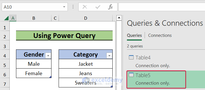
- A connection table sign will appear on the right side of the sheet.
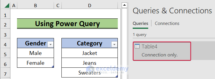
- Repeat the same steps for the Category table.
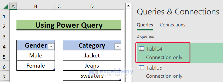
There will be two table connections.
- Choose Table4.
- The Power Query window will open.
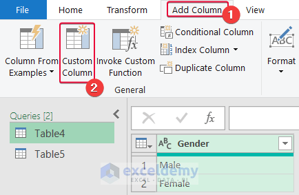
- Go to the Add Column.
- Select Custom Column.
- In the Custom Column prompt, enter Table5.
- Click OK.
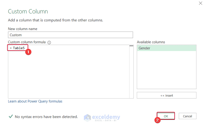
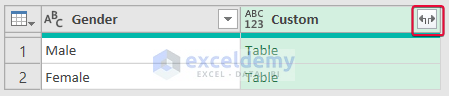
- The Custom column will be added beside the Gender column.
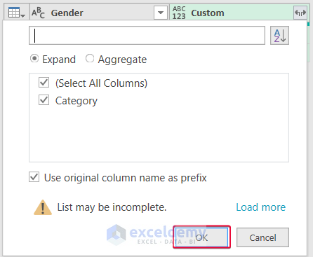
- Select the double arrow sign in the top right corner of the column.
- Select OK.
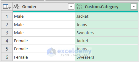
- The Category column will appear beside the Gender column.
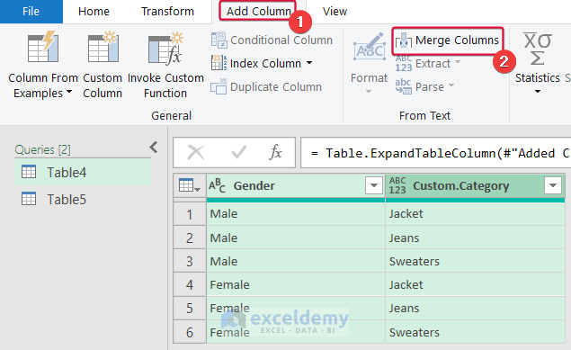
- Go to the Add Column tab.
- Select Merge Columns.
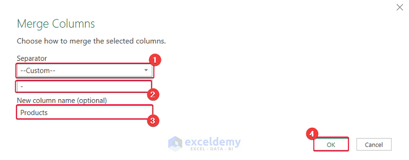
- A prompt will open on the screen.
- Select Custom.
- Type “-” as the separator.
- Rename the merged column as Products.
- Choose OK.
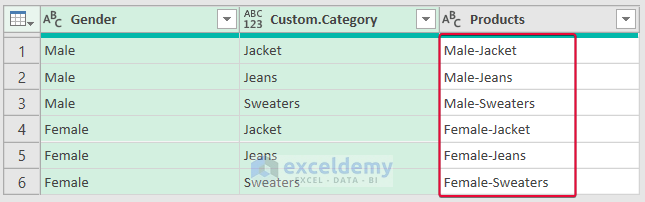
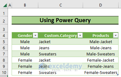
We will have all the combinations of the 2 columns in Power Query.
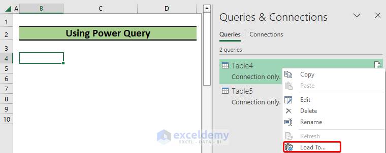
- Open a new worksheet.
- Go to the Data tab.
- Select Queries & Connections.
- The list of tables will appear on the right side of the sheet.

- Choose cell B4.
- Right-click on one of the tables.
- From the available options, select Load To.
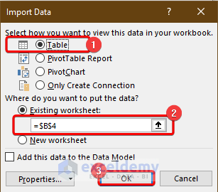
- A prompt will open on the screen.
- Select Table.
- Select cell B4 as the cell to insert the table.
- Click OK.
We will get all the combinations of the 2 columns.
Notes: Here, we could not use the Close & Load command to load the Power Query table in the Excel sheet because we created the tables by applying Connection Only. So, we had to transform it into the table before inserting it into an Excel sheet.
Method 2 – Applying Combined Excel Functions
Steps:
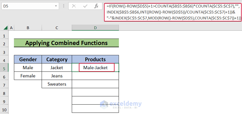
- Click on cell D5 and enter,
=IF(ROW()-ROW($D$5)+1>COUNTA($B$5:$B$6)*COUNTA($C$5:$C$7),"", INDEX($B$5:$B$6,INT((ROW()-ROW($D$5))/COUNTA($C$5:$C$7)+1))&"-"&INDEX($C$5:$C$7,MOD(ROW()-ROW($D$5),COUNTA($C$5:$C$7))+1))- Press Enter.
Formula Breakdown
- ROW()-ROW($D$5)+1>COUNTA($B$5:$B$6)*COUNTA($C$5:$C$7): Here, the ROW() returns the value of the row of the D5 cell which is So as the ROW($D$5). Now, the formula becomes 5-5+1>COUNTA($B$5:$B$6)*COUNTA($C$5:$C$7). The COUNTA($B$5:$B$6) and COUNTA($C$5:$C$7) return the number of non-empty cells in the range B5:B6 and C5:C7, which are 2 and 3 respectively. So the expression becomes 1>2*3 or 1>6, which is False.
- Output: False
- INDEX($B$5:$B$6,INT((ROW()-ROW($D$5))/COUNTA($C$5:$C$7)+1)): The (ROW()-ROW($D$5) returns The COUNTA($C$5:$C$7) expression counts the number of non-empty cell in the C5:C7 range and returns 3. So, the expression becomes INDEX($B$5:$B$6,INT(0/3+1)) and will become INDEX($B$5:$B$6,INT(0+1)) or INDEX($B$5:$B$6,INT(1)) . The INT function will return 1. The final expression will be INDEX($B$5:$B$6,1). Finally, the INDEX function will return the 1st value of the B5:B6 range, which is Male.
- Output: Male
- INDEX($C$5:$C$7,MOD(ROW()-ROW($D$5),COUNTA($C$5:$C$7))+1)): The MOD(ROW()-ROW($D$5),COUNTA($C$5:$C$7))+1 will become MOD(0,3)+1. The MOD function will return the remainder of the division between 0 and 3 which is So, the INDEX($C$5:$C$7,MOD(ROW()-ROW($D$5),COUNTA($C$5:$C$7))+1)) becomes INDEX($C$5:$C$7,0+1)) or INDEX($C$5:$C$7,1)). Thus, the expression will return the first value of the cell range C5:C7 and that will be Jacket.
- Output: Jacket
- IF(ROW()-ROW($D$5)+1>COUNTA($B$5:$B$6)*COUNTA($C$5:$C$7),””, INDEX($B$5:$B$6,INT((ROW()-ROW($D$5))/COUNTA($C$5:$C$7)+1))&”-“&INDEX($C$5:$C$7,MOD(ROW()-ROW($D$5),COUNTA($C$5:$C$7))+1)): This expression becomes IF(False,#NA, “Male” &”-“& “Jacket”). So, the expression is asking to concatenate the Male , – , and Jacket if the condition is
- Output: Male-Jacket
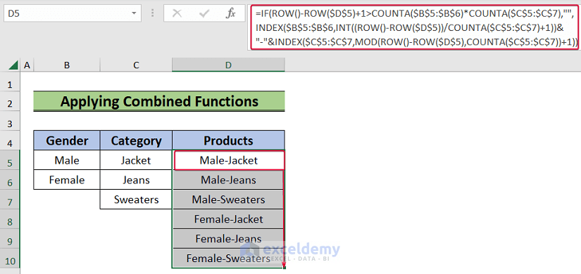
- We will have the first combination of the two columns.
- Drag the cursor down to autofill the rest of the cells.
Method 3 – Using Helper Columns and Combined Functions
Steps:
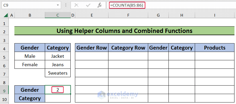
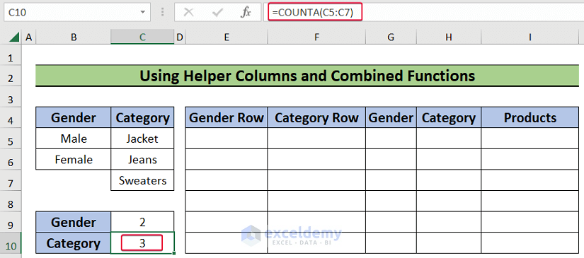
- Choose cell C9 and enter the following formula:
=COUNTA(B5:B6)- Press Enter.
- We will have the counting of the values in the Gender column.
- Select cell C10 and enter the following formula:
=COUNTA(C5:C7)- Press Enter.
- We will get the number of values under the Category column.
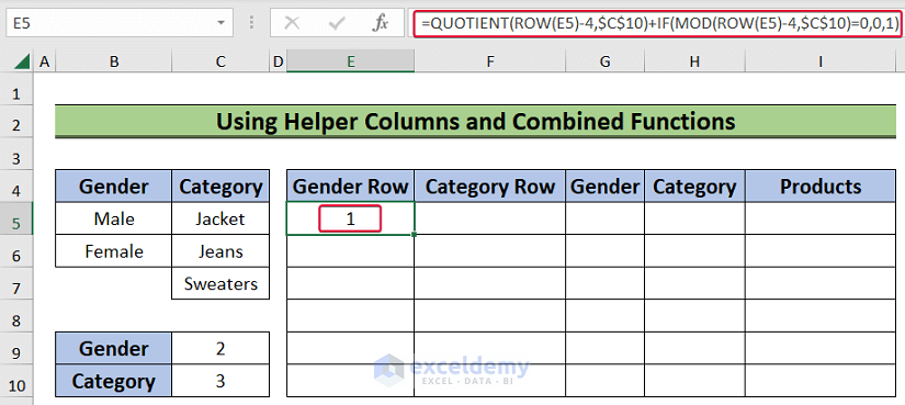
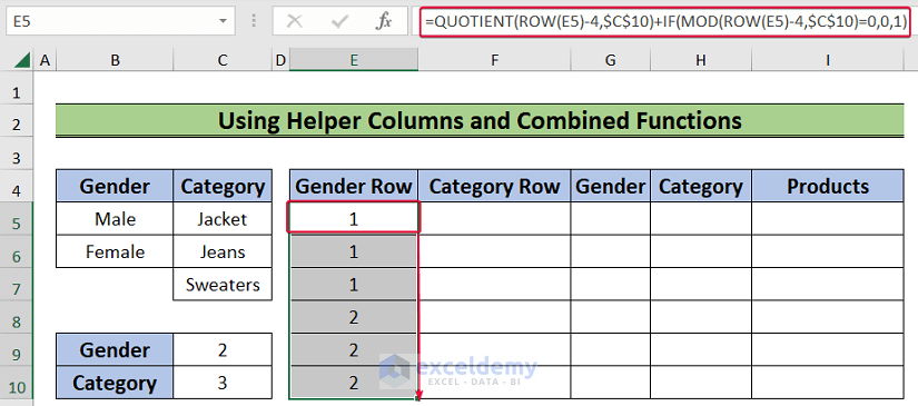
- Choose cell E5 and enter the following formula:
=QUOTIENT(ROW(E5)-4,$C$10)+IF(MOD(ROW(E5)-4,$C$10)=0,0,1)- Press Enter.
Formula Breakdown
- QUOTIENT(ROW(E5)-4,$C$10): The ROW(E5)-4 expression will become 5-4 or So the overall expression be QUOTIENT(1,$C$10) or QUOTIENT(1,3). The QUOTIENT function will return the integer part of the division of 1 by 3 which is 0.
- Output: 0
- IF(MOD(ROW(E5)-4,$C$10)=0,0,1): The ROW(E5)-4 expression will return The MOD(ROW(E5)-4,$C$10) will become MOD(1,3) which returns 1. So, the overall expression will be IF(1=0,0,1) or IF(False,0,1). Finally, the formula will return 1.
- Output: 1
- QUOTIENT(ROW(E5)-4,$C$10)+IF(MOD(ROW(E5)-4,$C$10)=0,0,1): The entire expression will become 0+1 or
- Output: 1
- We will assign the row number for the first value of the Gender column.
- Drag the cursor down and autofill the rest of the cells.
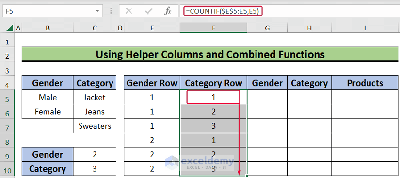
- Click on cell F5 and enter the following formula:
=COUNTIF($E$5:E5,E5)- Press Enter.
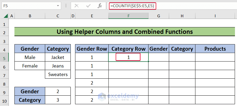
- We will get the row number for the first value of the Category column.
- Drag the cursor down to autofill.
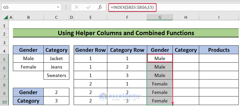
- Choose cell G5 and enter the following formula:
=INDEX($B$5:$B$6,E5)- Press Enter.
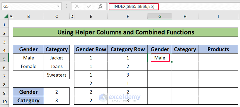
- We will have the first value of the Gender column associated with the value in the Gender Row.
- Drag the cursor to autofill the rest of the cells.
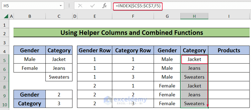
- Choose cell H5 and enter the following formula:
=INDEX($C$5:$C$7,F5)- Press Enter.
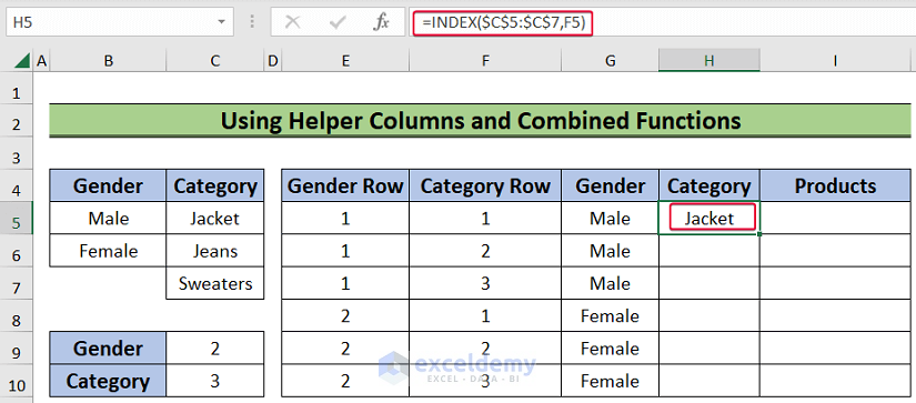
- We will have the first value of the Category column associated with the value in the Category Row.
- Drag the cursor down to the last cell to autofill.
- Choose cell I5 and enter the following formula:
=CONCATENATE(G5,"-",H5)- Press Enter.
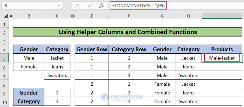
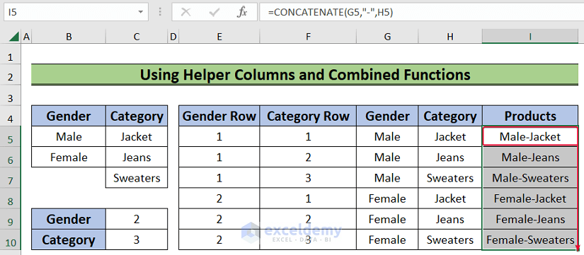
- We will have our first combination of the 2 columns.
- Drag the cursor to autofill the rest of the cells.
Method 4 – Applying VBA Code
Steps:
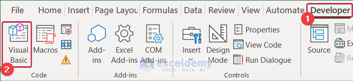
- Go to the Developer tab.
- Select the Visual Basic tab.
- A new window will open on the screen.
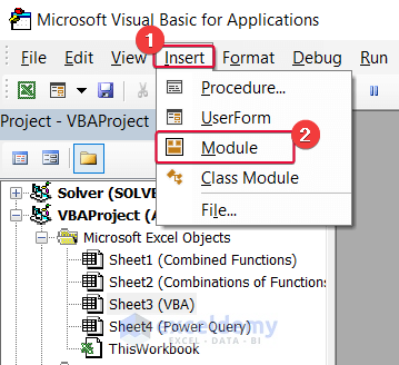
- From the Visual Basic window, select Insert.
- Choose Module from the drop-down list.
- A new module will appear.
- Enter the following formula and save it:
Sub AllCombinationsTwoColumns()
Dim am_r1, am_r2 As Range
Dim am_r  As Range
Dim am_str As String
Dim am_int1, am_int2 As Integer
Dim am_str1, am_str2 As String
Set am_r1 = Range("B5:B6")
Set am_r2 = Range("C5:C7")
am_str = "-"
Set am_r = Range("D5")
For am_int1 = 1 To am_r1.Count
    am_str1 = am_r1.Item(am_int1).Text
    For am_int2 = 1 To am_r2.Count
        am_str2 = am_r2.Item(am_int2).Text
        am_r.Value = am_str1 & am_str & am_str2
        Set am_r = am_r.Offset(1, 0)
       Next
    Next
End Sub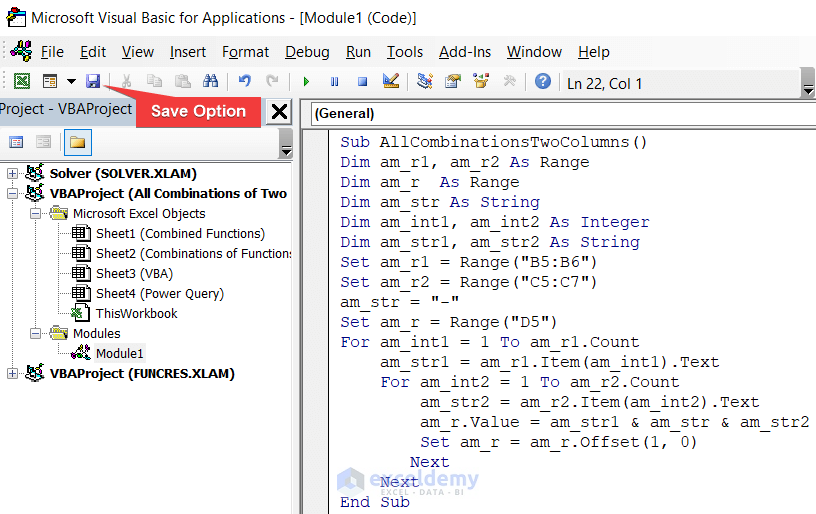
- Run the code by clicking on the triangular-shaped green button.
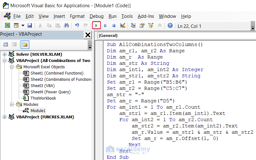
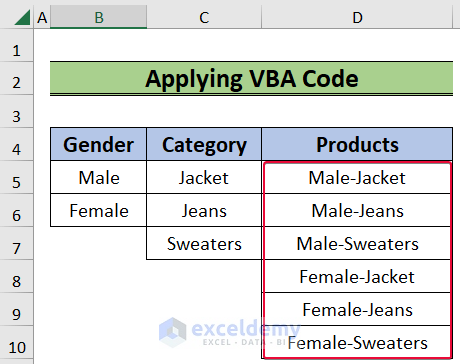
- We will have all the combinations of 2 columns in the D5:D10 cell range.
Download the Practice Workbook
You can download the practice workbook here.
Related Articles
- How to Sum All Possible Combinations in Excel
- How to Find Combinations Without Repetition in Excel
- How to Apply All Combinations of 3 Columns in Excel
- How to Create All Combinations of 4 Columns in Excel
- How to Show All Combinations of 5 Columns in Excel
- How to Create All Combinations of 6 Columns in Excel
<< Go Back to Excel COMBIN Function | Excel Functions | Learn Excel
Get FREE Advanced Excel Exercises with Solutions!
