How to Apply All Combinations of 3 Columns in Excel

Sometimes we need to find combinations of various things. Only a few different things can have a large number of combinations. As a result, finding these combinations manually would be painstaking and time-consuming. Therefore, we will use some tricks to find combinations in Excel easily. In this article, we will show you how to apply all combinations of 3 columns in Excel in 3 easy ways.

How to Apply All Combinations of 3 Columns in Excel: 3 Effective Ways

In this article, we will demonstrate 3 effective ways to apply all combinations of 3 columns in Excel. We will use the following dataset for this purpose.

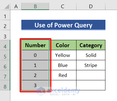
1. Use Power Query

In this method, we will use the Power Query Feature to apply all combinations of 3 columns. The procedure is discussed below.

Steps:

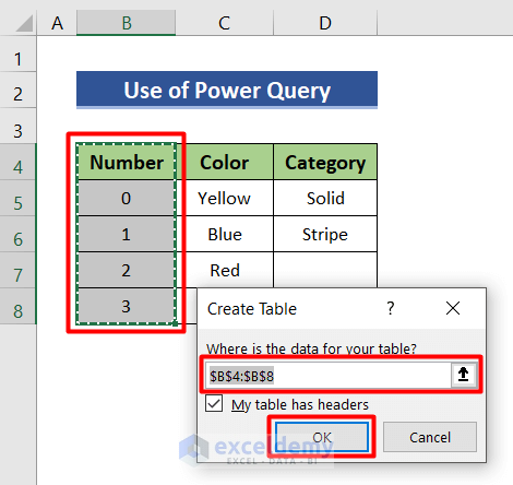
First, we need to create 3 separate tables for 3 columns. To do that, select the first column and press Ctrl+T.

Create Table window will appear. Now Press Enter.

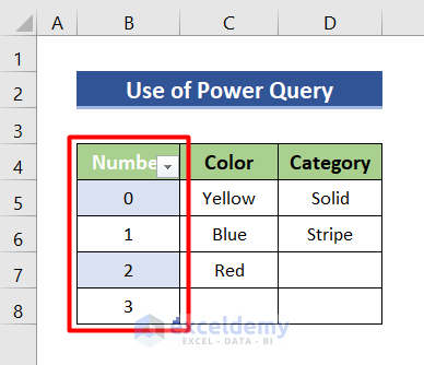
The Number column is now turned into a table.

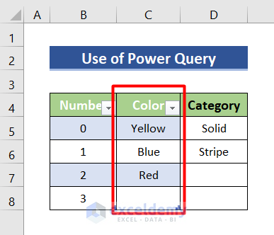
Similarly, we will make the Color column a table. For that, select the Color column.

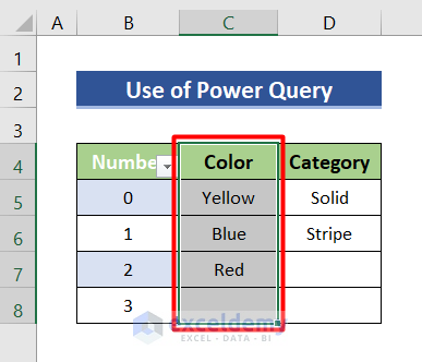
Then press Ctrl+T.
After that, press Enter.

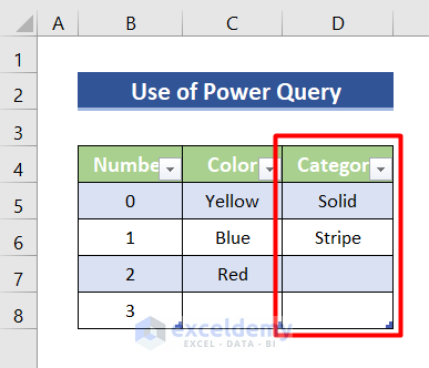
Following the same process, turn the last column into a table too.

Now we need to create a connection for each column.
For that, go to the Data tab and select From Table/Range.

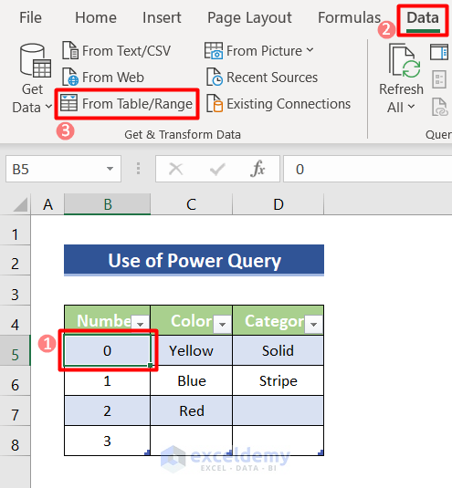
Power Query Editor window will open with the data of the first column.

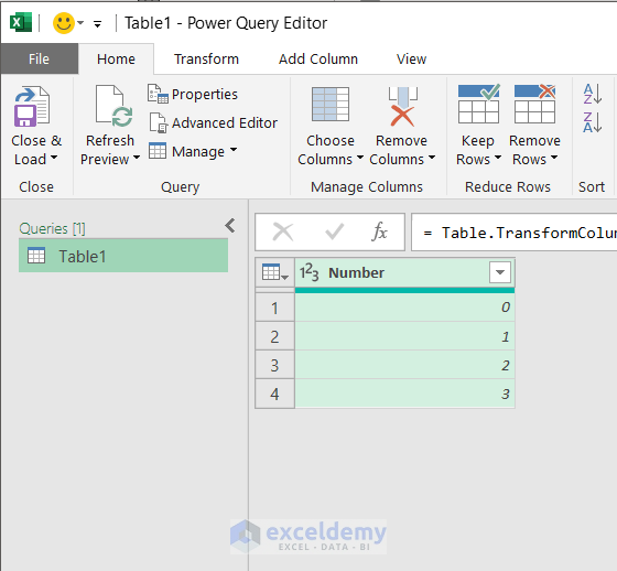
Next, right-click on Table1 and click on Rename.

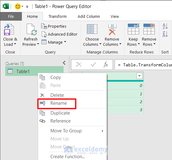
Now rename the table. We renamed it Number.

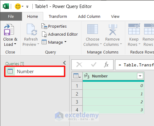
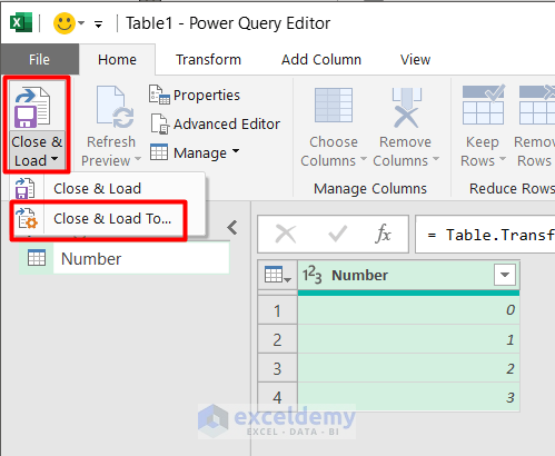
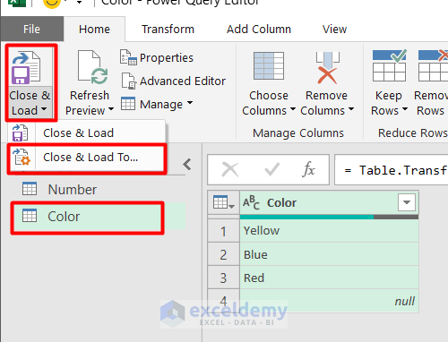
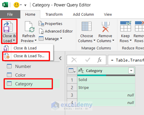
Next, in the Home tab, click on Close & Load.
Then select Close & Load To.

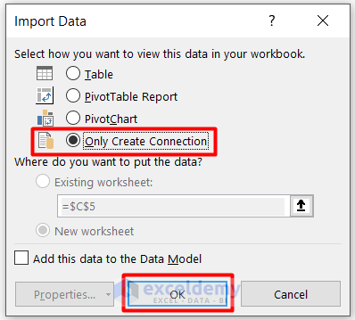
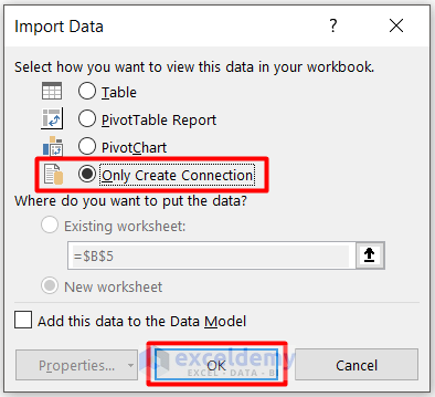
A dialogue box will open. Select Only Create Connection there and press OK.

Now follow the exact same procedure to add the Color column in Power Query Editor.

Then create a connection for this column as well.

For the category column, again follow all the steps to add it to Power Query Editor.

Then create a connection in the Import Data dialogue box.

Now we will create temporary columns.
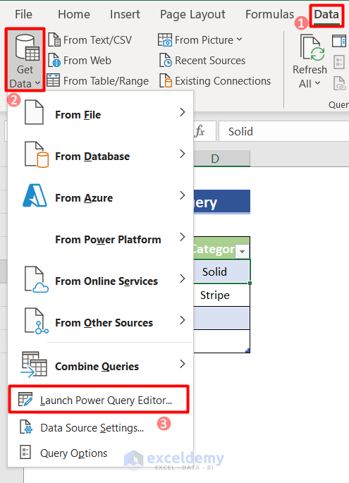
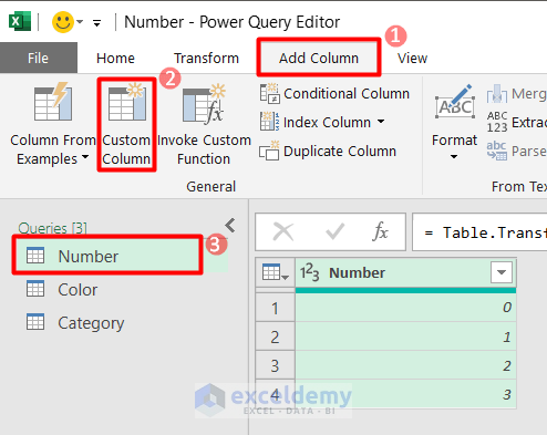
Click on Get Data in the Data From there, select Launch Power Query Editor.

Next, select the Number Then go to Add Column and click on Custom Column.

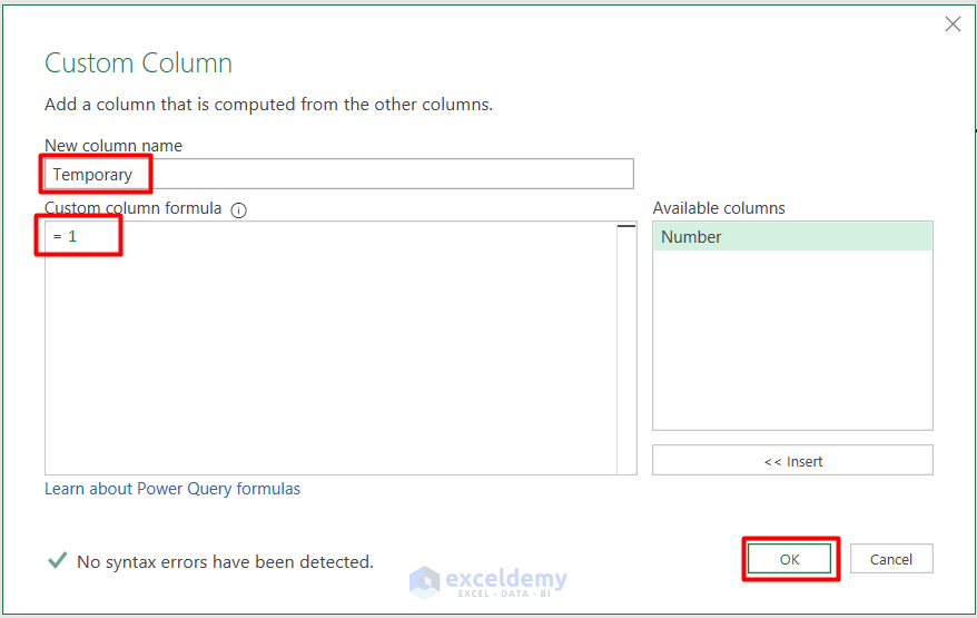
Create a column name for the new helper column. We named it Temporary.
In the custom column formula, write “= 1”.
This column name and formula must be the same for all 3 columns.

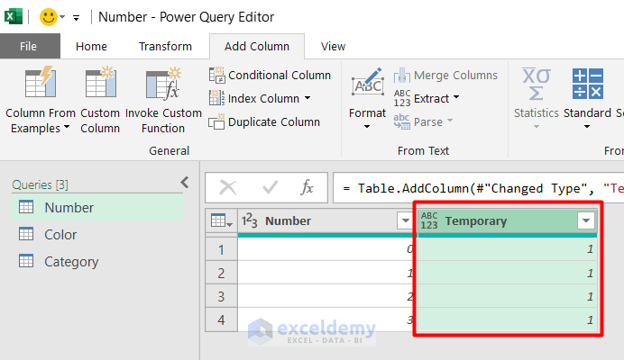
Press OK and you will see a temporary column beside the Number column.

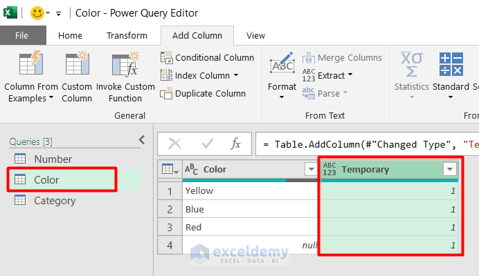
Similarly, create a temporary column beside the Color column.

Follow the same procedure for the Category column too.

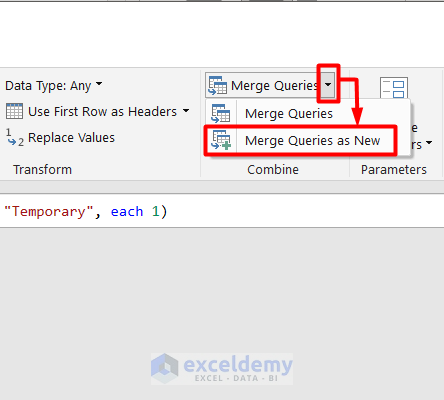
Now it’s time to merge the columns.
To do that, click on Merge Queries. Then select Merge Queries as New.

A pop-up box will appear. In the pop-up, choose the Number and the Color column and select the Temporary column.
Next, select Full Outer (all rows from both) in the Join Kind option.
Then click on OK.

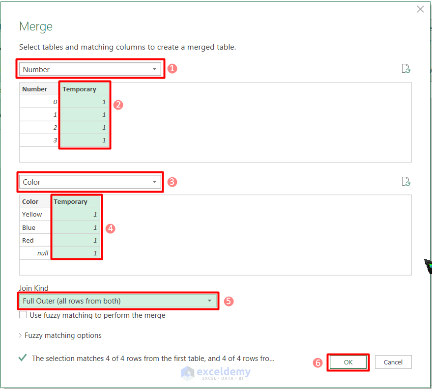
Now you will find that the Number and the Color table are merged and it is saved as Merge1.

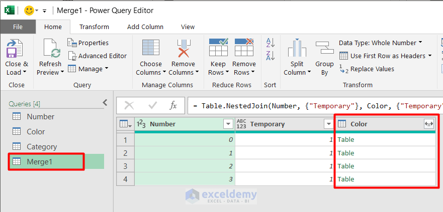
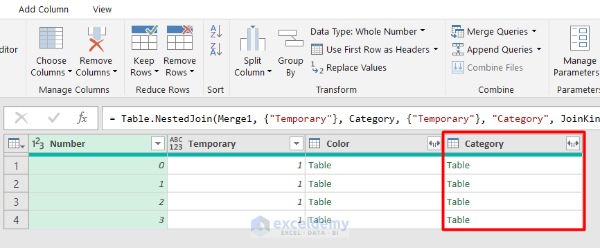
Now we will merge the Category table with the Merge1 table.
Choose Merge1 and Category and select the Temporary column.
Then select Full Outer (all rows from both) in the Join Kind option and hit Enter.

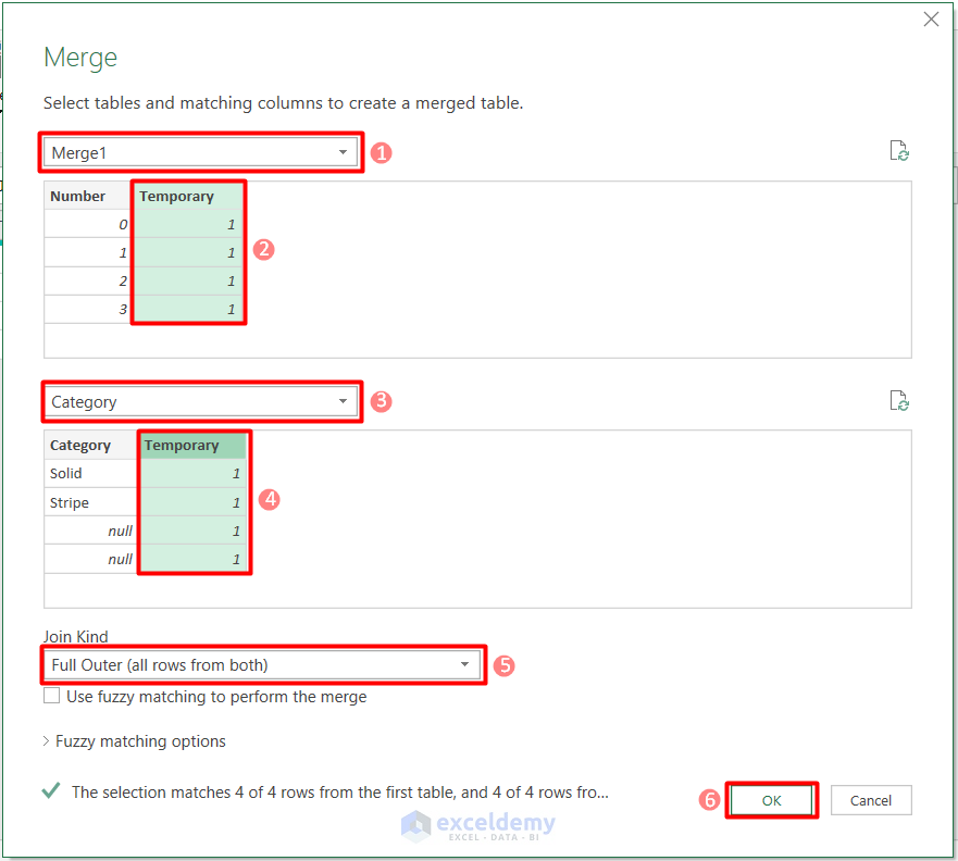
Now you can see that all three columns are merged together with the Temporary column.

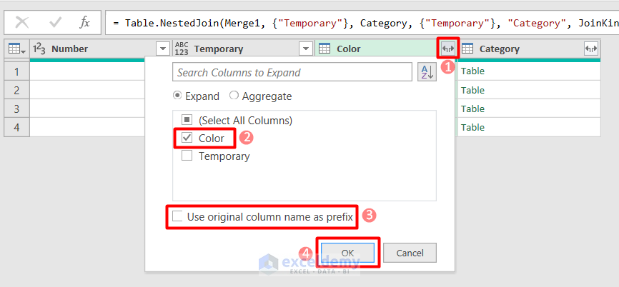
We will now find all the combinations of these 3 columns.
Click on the Color drop-down and select the Color option to expand the combinations.
Uncheck the box of Use original column name as prefix.
Press the Enter button.

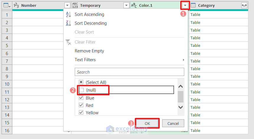
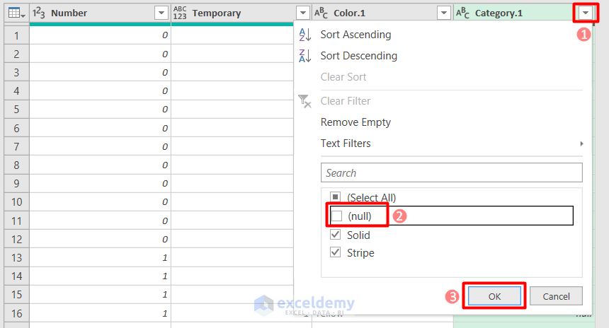
Next, click on the Color.1 drop-down.
Then uncheck the box of null.

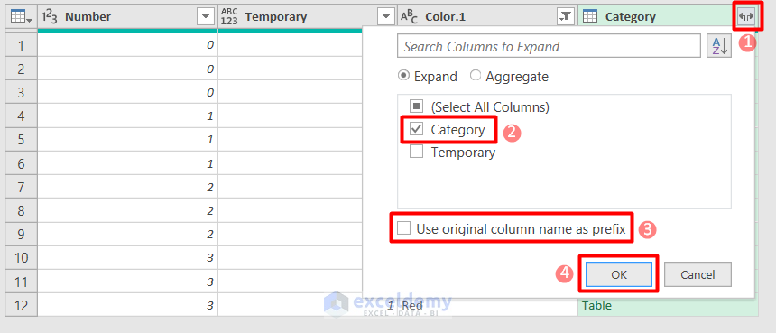
Follow the same steps for Category to expand the combinations and remove null rows.

Unchecking null removes the empty rows in the combinations.

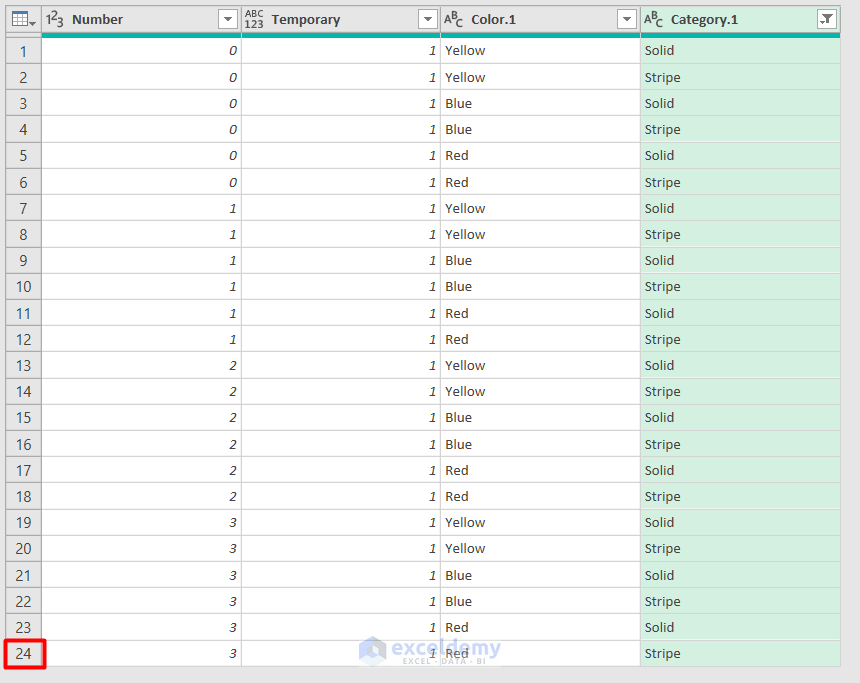
Finally, there you have all 24 combinations of the 3 columns.

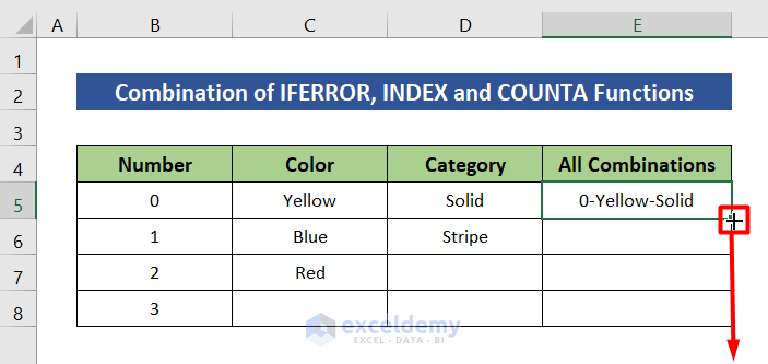
2. Combination of IFERROR, INDEX, and COUNTA Functions

We will combine the IFERROR, INDEX, and COUNTA functions to apply combinations of 3 columns. Follow these steps to learn.

Steps:

First of all, create a column named All Combinations.
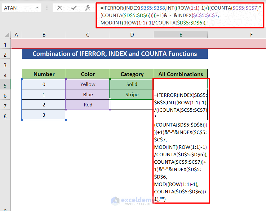
After that, type the following formula in cell E5.

=IFERROR(INDEX($B$5:$B$8,INT((ROW(1:1)-1)/((COUNTA($C$5:$C$7)* (COUNTA($D$5:$D$6)))))+1)&"-"&INDEX($C$5:$C$7, MOD(INT((ROW(1:1)-1)/COUNTA($D$5:$D$6)), COUNTA($C$5:$C$7))+1)&"-"&INDEX($D$5:$D$6, MOD((ROW(1:1)-1),COUNTA($D$5:$D$6))+1),"")

Formula Breakdown

• COUNTA($D$5:$D$6))+1) looks into cells D5 and D6 and counts the number of information.

INDEX($D$5:$D$6,MOD((ROW(1:1)-1),COUNTA($D$5:$D$6))+1) returns a value or the reference to a value from cell D5 to D6.

• INT((ROW(1:1)-1)/((COUNTA($C$5:$C$7)*(COUNTA($D$5:$D$6)))))+1) returns an integer value after dividing the number of “rows-1” by the product of the number of information in cell C5 to C7 and D5 to D7.

• =IFERROR(INDEX($B$5:$B$8,INT((ROW(1:1)-1)/((COUNTA($C$5:$C$7)*(COUNTA($D$5:$D$6)))))+1) evaluates the formula and returns all possible combinations.

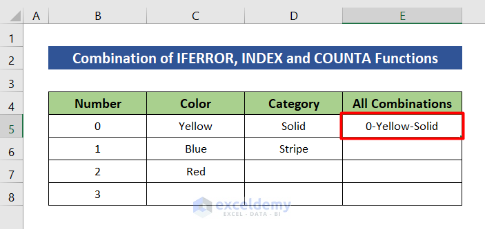
Press Enter and you will see the first combination.

Now drag the bottom right corner of cell E5 to copy the formula to all of the cells.

Once all the combinations are complete, you will start getting empty cells. You can just stop dragging when you get the first empty cell.

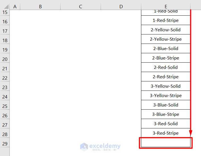
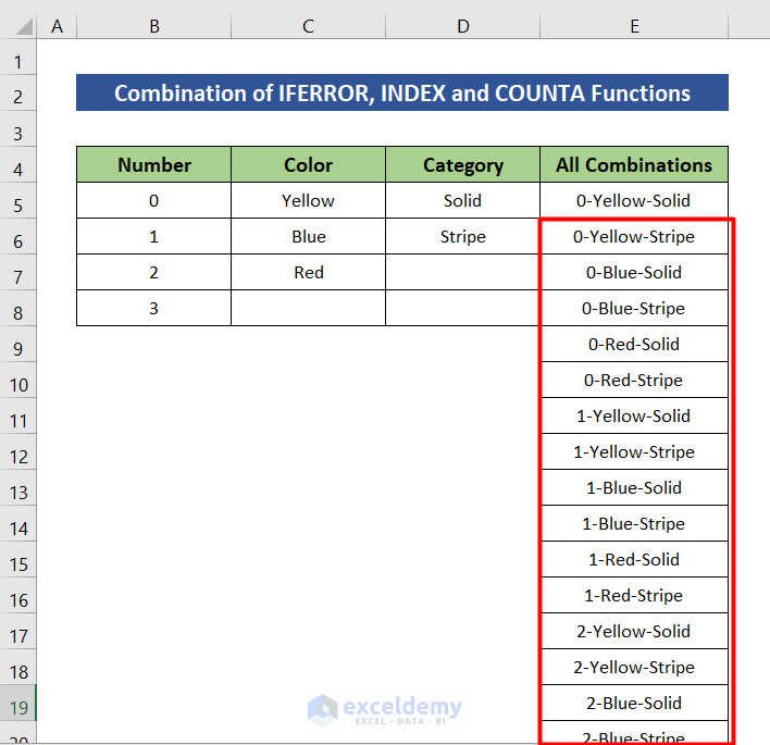
As can be seen, you will find all the combinations of the 3 columns in your Excel sheet.

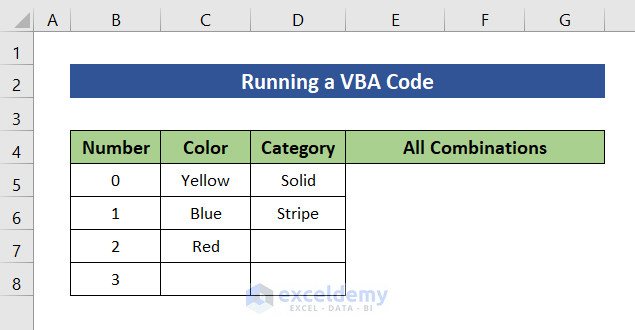
3. Run a VBA Code

Now we will run a VBA code to apply all combinations of 3 columns in Excel. Keep on reading to learn how to do it.

Steps:

First, create a column named All Combinations.

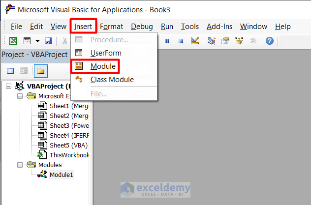
Now press Alt+F11 to open Microsoft Visual Basic window.

Then select Module in the Insert tab to open a module.

After that, copy the following VBA code in the module.

Sub AllCombinations()
    i = 5
    For Each cella In ThisWorkbook.ActiveSheet.Range("B5:B8")
    .SpecialCells (xlCellTypeConstants)
    For Each cellb In ThisWorkbook.ActiveSheet.Range("C5:C7")
    .SpecialCells (xlCellTypeConstants)
    For Each cellc In ThisWorkbook.ActiveSheet.Range("D5:D6")
    .SpecialCells (xlCellTypeConstants)
    ThisWorkbook.ActiveSheet.Range("E" & i).Value = cella.Value
    ThisWorkbook.ActiveSheet.Range("F" & i).Value = cellb.Value
    ThisWorkbook.ActiveSheet.Range("G" & i).Value = cellc.Value
    i = i + 1
    Next
    Next
    Next
End Sub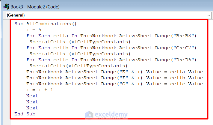

Then press F5 to run the VBA code.
Lastly, go back to the worksheet and get all the combinations of three columns.

Things to Remember

Don’t forget to give proper cell references or you won’t get the desired results.
Make sure that the temporary column in the Power Query has the same name for all 3 columns.

Download Practice Workbook

Download this practice workbook for practice while you are reading this article.

All Combination of 3 Columns.xlsm

Concluding Remarks

Thanks for making it this far. I hope you find this article useful. Now you know 3 different methods to apply all combinations of 3 columns in Excel. Please let us know if you have any further queries and feel free to give us any recommendations in the comment section below.

<< Go Back to Excel COMBIN Function | Excel Functions | Learn Excel

Get FREE Advanced Excel Exercises with Solutions!

How to Apply All Combinations of 3 Columns in Excel

How to Apply All Combinations of 3 Columns in Excel: 3 Effective Ways

1. Use Power Query

2. Combination of IFERROR, INDEX, and COUNTA Functions

3. Run a VBA Code

Things to Remember

Concluding Remarks

Related Articles

Leave a reply Cancel reply