How to Count Cells in Excel with Different Text: 5 Methods

Method 1 – Applying SUM & COUNTIF to Count Cells in Excel with Different Text

STEPS:

➤ In cell E4, type the following formula.

=SUM(1/COUNTIF(B4:B13,B4:B13))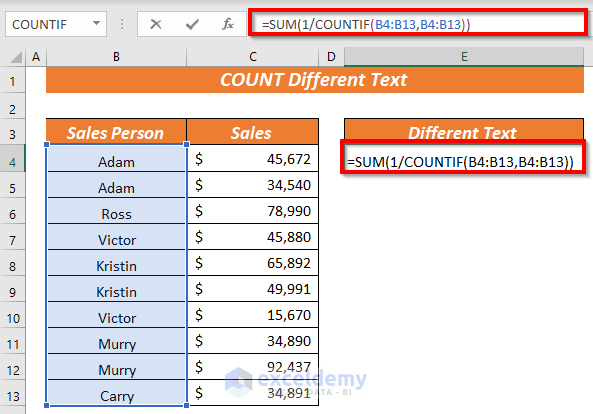

Formula Breakdown

➦ COUNTIF(B4:B13,B4:B13) —> Get you how many times each individual value appears in the specified range.
Output : {2;2;1;2;2;2;2;2;2;1}

➦ 1/COUNTIF(B4:B13,B4:B13) —> Reciprocates the output of previous steps.
Output : {0.5;0.5;1;0.5;0.5;0.5;0.5;0.5;0.5;1}

➦ SUM(1/COUNTIF(B4:B13,B4:B13)) —> Sums the values 0.5,0.5,1,0.5,0.5,0.5,0.5,0.5,0.5,1.
Output: {6}

➤ Press CTRL + SHIFT + ENTER If you are not using Microsoft Office 365. Get the number of different text in the range B4:B13.

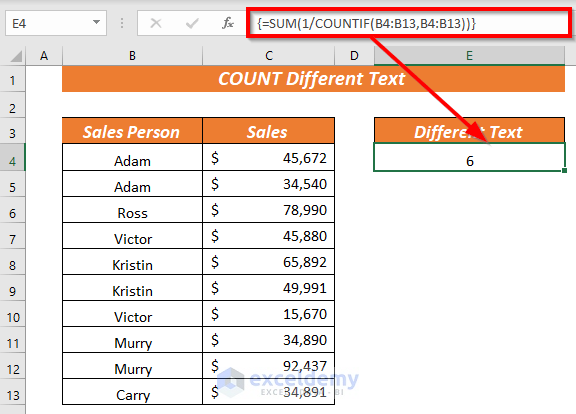
Note: Please remember that you have to press CTRL + SHIFT + ENTER as it is an array formula. Notice the curly bracket ‘{}’ in the formula bar that denotes an array formula.

Method 2 – Use of Pivot Table to Count Cells in Excel with Different Text

STEPS:

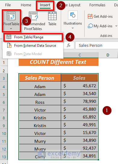
➤ Create a Pivot Table with the dataset. Select the range B3:C13 >> go to Insert Tab >> select Pivot Table >> select From Table/Range.

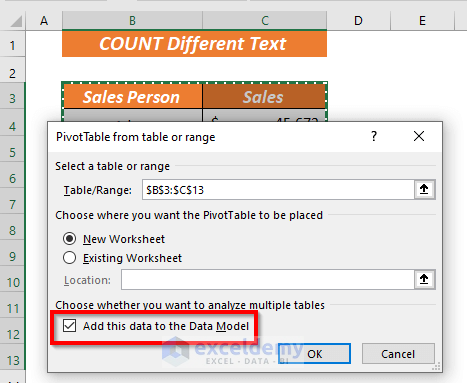
➤ PivotTable from table or range window will appear. Add this data to the Data Model box. Press OK.

Create a Pivot Table for you.
➤ Put Sales Person in the Rows Field and Values Field. Excel will by default show you the count of Sales Person on the left side.

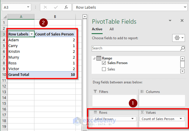
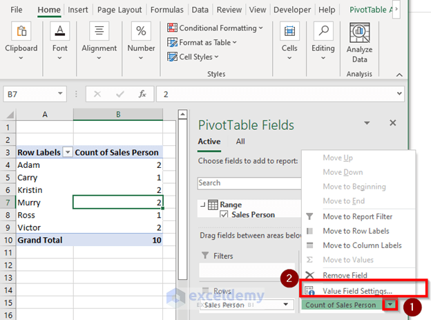
➤ Click the drop-down list of Count of Sales Person from the Value Field and select Value Field Settings.

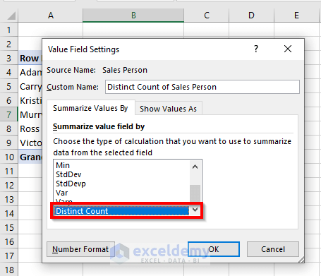
➤ Value Field Settings dialog box will pop up. Choose Distinct Count as the type of calculation. Click OK.

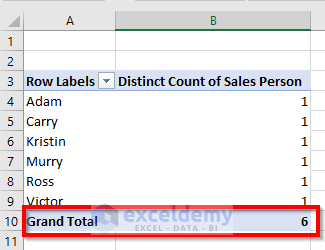
➤ Excel will show you the total number of cells have different texts.

Method 3 – Using a User Defined Functions to Count Different Text Ignoring Blank Cells

STEPS:

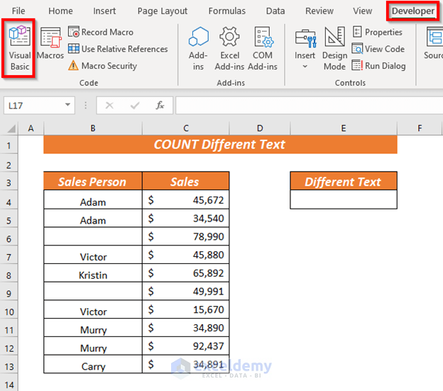
➤ Go to Developer tab >> select Visual Basic.

➤ Go to Insert tab >> select Module.

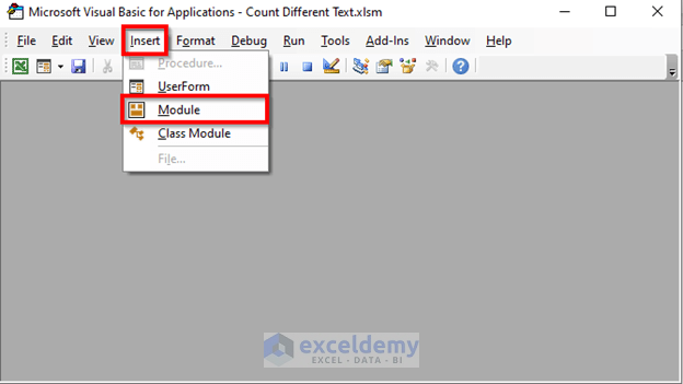
Module window will show up. Write down the following code

Function COUNTDIFFERENT(DataRange As Range, CountBlanks As Boolean) As Integer
Dim CellContent As Variant
Dim DifferentValues As New Collection
Application.Volatile
On Error Resume Next
For Each CellContent In DataRange
If CountBlanks = True Or IsEmpty(CellContent) = False Then
DifferentValues.Add CellContent, CStr(CellContent)
End If
Next
COUNTDIFFERENT = DifferentValues.Count
End Function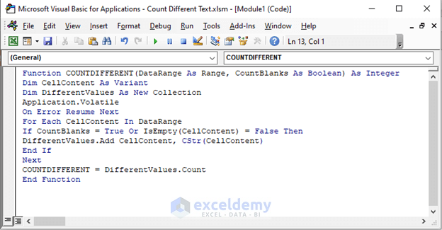

We created a new Function COUNTDIFFERENT. The function has two arguments, DataRange and CountBlanks. They are set as Range and Boolean. The outcome or result of the function COUNTDIFFERENT will be in Integer form.
We declared two variables using Dim Statement these are CellContent, and DifferentValues as Variant and New Collection.
We used a for loop to check whether there are any Blank cells in the selected cell range.
We used the IF statement to count or not count Blank Cells as Different Text. If the Boolean is TRUE, Excel will show the number of different text including the blank cells, it will ignore the blank cells in case the Boolean is FALSE.
➤ Save the program. The function is ready to use.
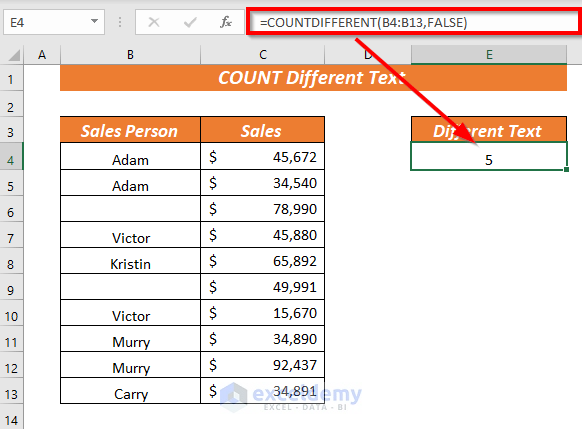
➤ Go back to your existing Workbook. Select cell E4 and write down the following formula-

=COUNTDIFFERENT(B4:B13,FALSE)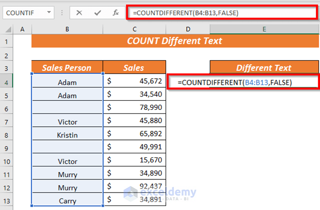

We selected the range B4:B13 and selected the Boolean FALSE as we wanted to ignore the blank cells.
➤ Press ENTER. Excel will return you the number of cells with different text ignoring the blank ones.

Method 4 – Using Combined Functions to Count Distinct Texts

STEPS:

In cell E4, type the following formula.

=SUM(IF(ISTEXT(B4:B13)*COUNTIF(B4:B13,B4:B13)=1,1,0))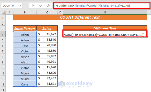

Formula Breakdown

➦ COUNTIF(B4:B13,B4:B13) —> It determines how many times the values in the selected range appear respectively.
Output : {2;2;1;2;2;2;2;2;2;1}

➦ ISTEXT(B4:B13) —> Declares whether the values in the selected range are Text or not.
Output : {TRUE;TRUE;TRUE;TRUE;TRUE;TRUE;TRUE;TRUE;TRUE;TRUE}

➦ ISTEXT(B4:B13)*COUNTIF(B4:B13,B4:B13) —> This is the logical test. Boolean TRUE represents 1, and FALSE represents 0.
Output: {2;2;1;2;2;2;2;2;2;1}

➦ IF(ISTEXT(B4:B13)*COUNTIF(B4:B13,B4:B13)=1,1,0) —> This returns the result by analyzing the logical test.
➦ IF({2;2;1;2;2;2;2;2;2;1}=1,1,0)
Output: {0;0;1;0;0;0;0;0;0;1}

➦ SUM(IF(ISTEXT(B4:B13)*COUNTIF(B4:B13,B4:B13)=1,1,0)) —> Determines the sum of the previous outputs.
➦ SUM({0;0;1;0;0;0;0;0;0;1})
Output: {2}

➤Press CTRL + SHIFT + ENTER. Excel will return the result.

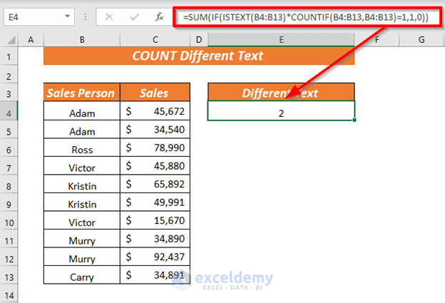
The result is 2 now. That’s because only Ross and Carry are the distinct texts. That means they are present only once in the range.

Method 5 – Count Different Text ignoring Numeric or Date Values

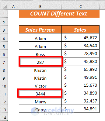
If you have different types of values (for instance, Date or Number) in a column and just want to count the Different Text, you can use the ISTEXT and IF functions along with the SUM and COUNTIF functions.
Notice that we put two numbers intentionally in cells B7 and B11.

STEPS:

➤ In cell E4, type the following formula.

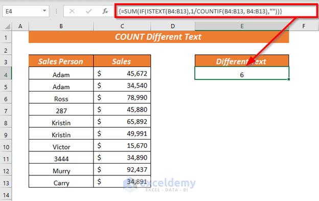
=SUM(IF(ISTEXT(B4:B13),1/COUNTIF(B4:B13, B4:B13),""))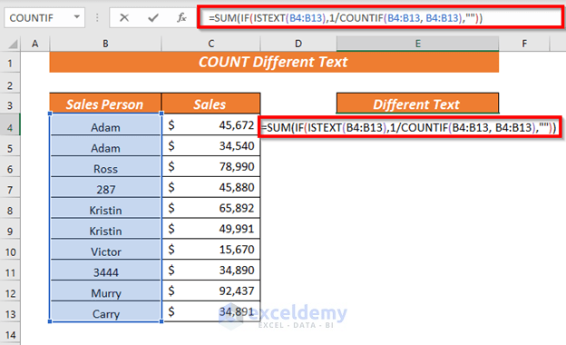

Formula Breakdown

➦ COUNTIF(B4:B13,B4:B13) —> Determines how often the values in the selected range appear respectively.
Output : {2;2;1;1;2;2;1;1;1;1}

➦ 1/COUNTIF(B4:B13,B4:B13) —> Determines the reciprocals of 2,2,1,1,2,2,1,1,1,1
Output : {0.5;0.5;1;1;0.5;0.5;1;1;1;1}

➦ ISTEXT(B4:B13) —> Declares whether the values in the selected range are Text or not.
Output : {TRUE;TRUE;TRUE;FALSE;TRUE;TRUE;TRUE;FALSE;TRUE;TRUE}

➦ IF(ISTEXT(B4:B13),1/COUNTIF(B4:B13, B4:B13),””) —> Returns the output analyzing the logical test.
Output : {0.5;0.5;1;””;0.5;0.5;1;””;1;1}

➦ SUM(IF(ISTEXT(B4:B13),1/COUNTIF(B4:B13, B4:B13),””)) —> Determines the sum of the previous outputs.
Output : {6}

➤ Press CTRL + SHIFT + ENTER. Excel will return you the number of different text ignoring other types of values.