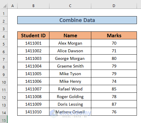
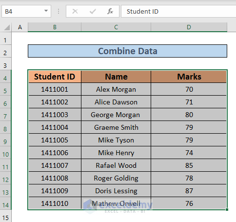
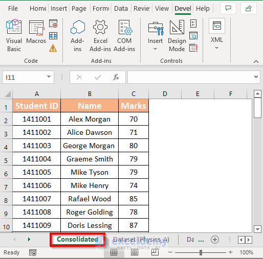
We have several students along with their Student ID and their Marks, where each sheet contains values for a different subject. We’ll consolidate the Marks for different subjects.
Method 1 – Applying the Consolidate Feature to Combine Data from Multiple Excel Sheets
We will add the scores in Physics and Math for each student.
STEPS:
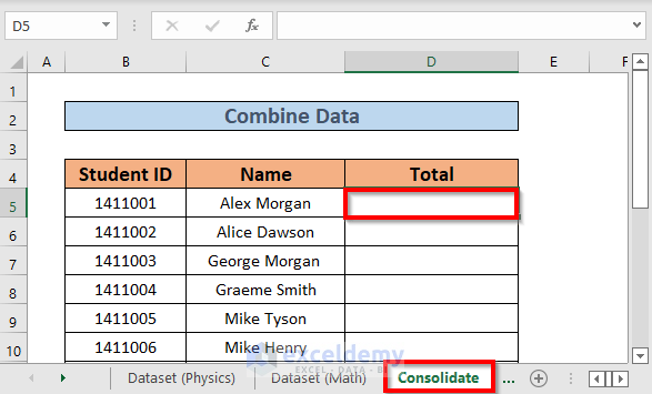
- We’ve made a new worksheet, Consolidate, and copied over the information for Student IDs and Names from the other sheets.
- Go to the Consolidate worksheet and select D5.
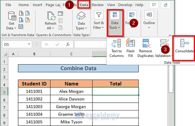
- Go to the Data tab and select Consolidate.
- A dialog box for Consolidate will appear.
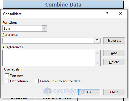
- Keep the Function drop-down as is since we’re summing the values.
- Click on the search arrow for Reference.
- Go to the Dataset (Physics) worksheet and select the range D5:D14.
- Select Add.
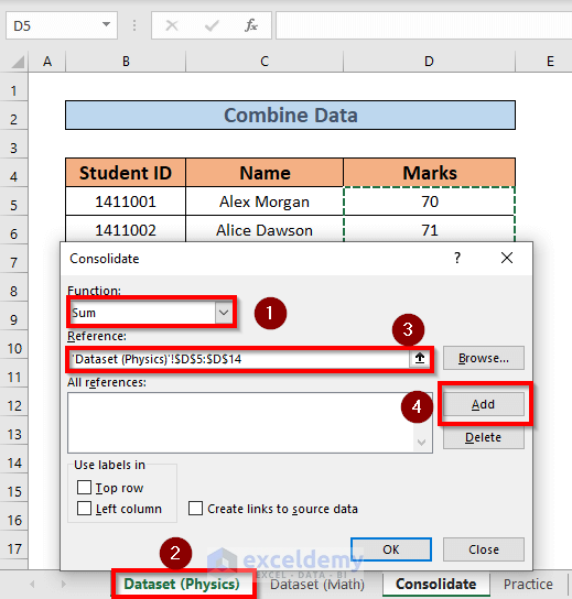
- Add the reference for the range D5:D14 from the Dataset (Math) workbook.
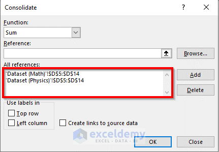
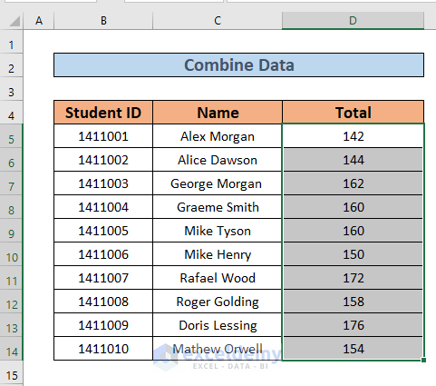
- Click OK. Excel will combine them and return the sum as output.
Method 2 – Using Excel Power Query to Combine Data from Multiple Sheets
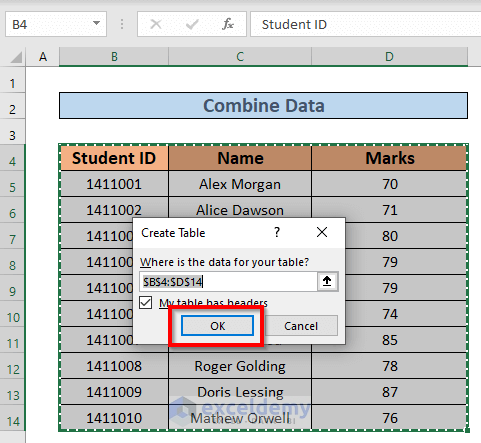
STEP 1 – Creating Tables
- Select the range B4:D14.
- Press Ctrl + T.
- The Create Table dialog box will pop up.
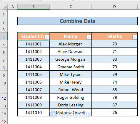
- Click OK.
- Excel will create the table.
- Go to the Table Design tab and rename the table.
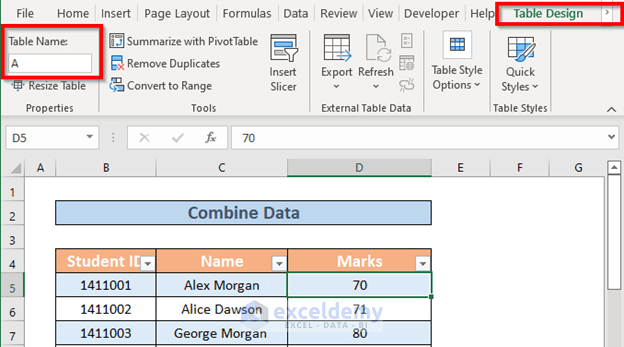
Repeat to create tables for all datasets.
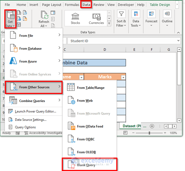
STEP 2 – Combine Data
- Go to the Data tab, select Get Data, choose From Other Sources, and select Blank Query
- The Power Query Editor window will appear. In the formula bar, use the formula:
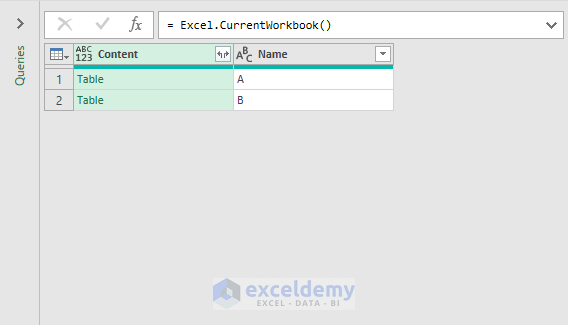
=Excel.CurrentWorkbook() 
- Press Enter. Excel will show the tables in your workbook.
- Click the double-headed arrow (see image).
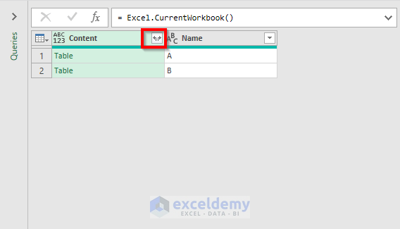
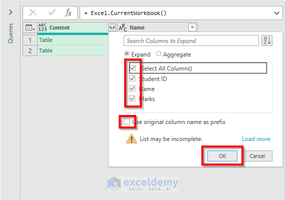
- Select the columns that you want to combine. We will combine all of them.
- Leave the Use original column name as prefix unmarked.
- Click OK.
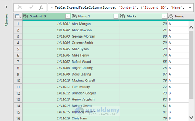
- Excel will combine the datasets.
- Select Close & Load.
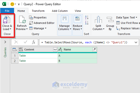
- Excel will create a new table combining the datasets.

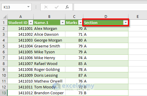
- Rename the Name column. We’re going to call this Section.
NOTE:
When you use the above method, you may face a problem.
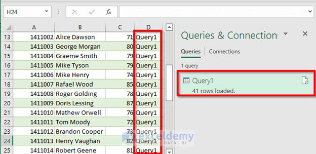
Our new table’s name is Query1 which consists of 21 rows including the headers.
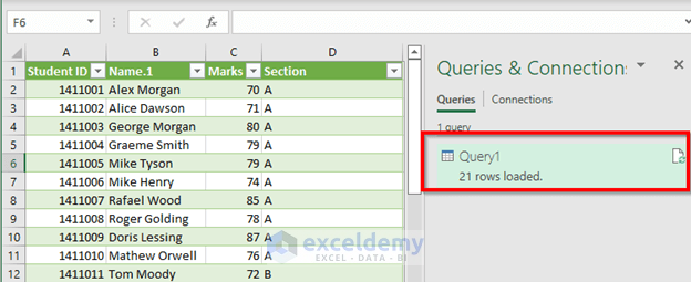
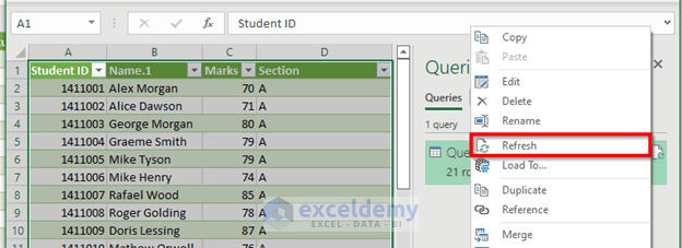
- Right-click to bring up the Context Menu and click Refresh.
- Once you refresh, you will see that the row number has changed to 41. That’s because Query1 itself is a table and is working as input.
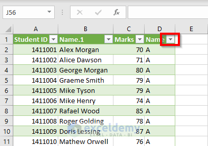
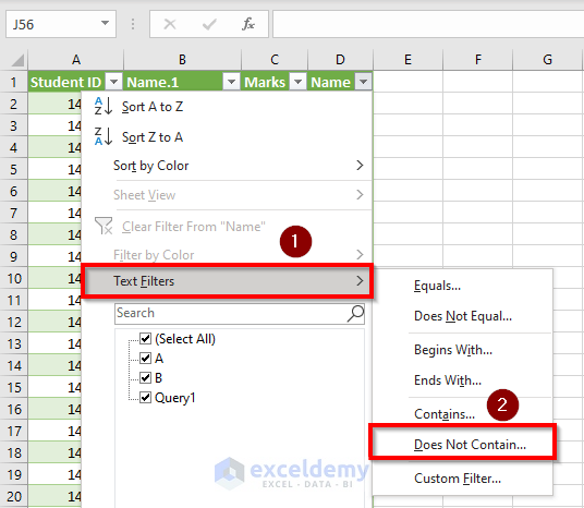
- Go to the drop-down of the column Name.
- Go to Text Filters and select Does Not Contain.
- A Custom AutoFilter window will open. Write Query1 in the box (see image).
- Click OK.
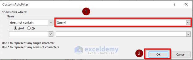
- The rows having the name Query1 will not be seen even if you refresh the dataset.
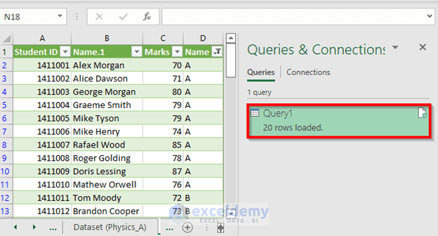
- 20 rows are loaded now because Excel is not counting the header this time.
Method 3 – Combining Data from Multiple Sheets Using VBA Macro
We have two worksheets, Dataset (Physics_A) and Dataset (Physics_B). We’ll combine the data from these datasets into a new worksheet named Consolidate.
STEPS:
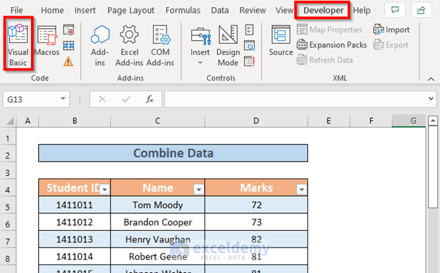
- Go to the Developer tab and select Visual Basic.
- Go to the Insert tab and Module.
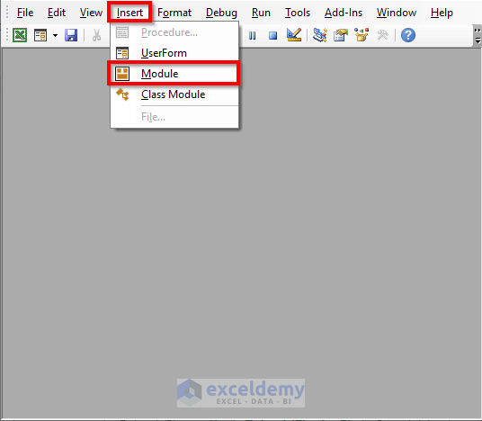
- A Module window will appear. Insert the following code.
Sub combine_multiple_sheets()

Dim Row_1, Col_1, Row_last, Column_last As Long
Dim headers As Range

Set wX = Worksheets("Consolidated")
Set WB = ThisWorkbook
Set headers = Application.InputBox("Choose the Headers", Type:=8)
headers.Copy wX.Range("A1")

Row_1 = headers.Row + 1
Col_1 = headers.Column
Debug.Print Row_1, Col_1

For Each ws In WB.Worksheets

If ws.Name <> "Consolidated" Then
ws.Activate
Row_last = Cells(Rows.Count, Col_1).End(xlUp).Row
Column_last = Cells(Row_1, Columns.Count).End(xlToLeft).Column
Range(Cells(Row_1, Col_1), Cells(Row_last, Column_last)).Copy _
wX.Range("A" & wX.Cells(Rows.Count, 1).End(xlUp).Row + 1)
End If

Next ws
Worksheets("Consolidated").Activate

End Sub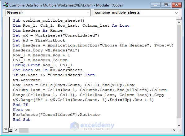
- Press F5 to run the program. Excel will create a combined dataset.
NOTE:
This VBA code will combine all the sheets available in your workbook indiscriminately. Make sure that your datasets follow the same formatting.
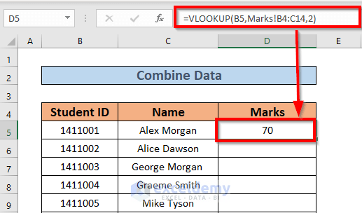
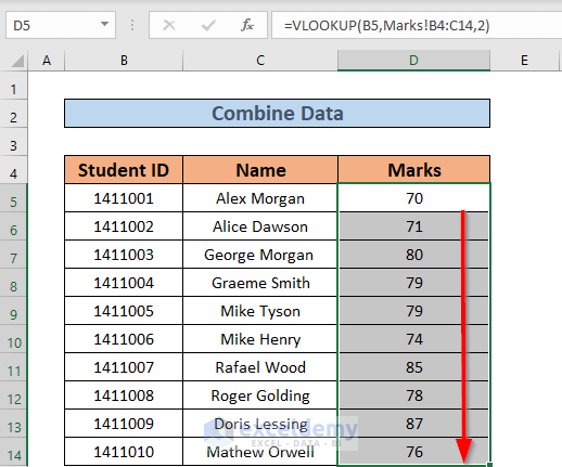
Method 4 – Inserting the VLOOKUP Function to Combine Data from Multiple Sheets
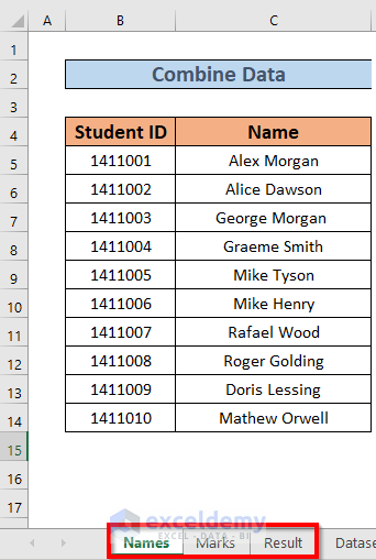
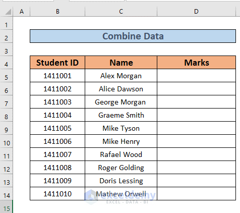
We have a worksheet named Names where we have the names of some students and another one named Marks. The sheets share the Student ID column. We’ll create a proper Result sheet by combining them.
Steps:
- Create a new column Marks after Names.
- Go to D5 and insert the following formula
=VLOOKUP(B5,Marks!B4:C14,2)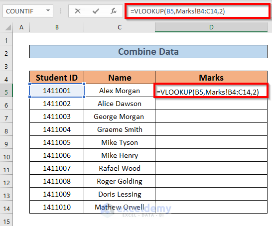
We have set the lookup value to B5 and the array is B4:C14 from the Marks sheet. The col_ind_num is 2 as we want the marks.
- Press Enter. Excel will return the output.
- Use the Fill Handle to AutoFill down to D14. Excel will extract the marks from the Marks worksheet for each student.
Download the Practice Workbook
<< Go Back To Merge Sheets in Excel | Merge in Excel | Learn Excel
Get FREE Advanced Excel Exercises with Solutions!

Power query is the replacment to MSQuery. I was au fait with MSQ but after a number of years have not managed to get to grips with Power Query. What I want to do is quite simple: to join two tables into one data set. This is more than just dump them into one query/table as they have different yet related data, along the lines of your student ID master file holding student names etc. I could use VLOOKUP() but I don’t want tens of thousands of additional formulae. I am avoiding using Access which is perhaps the obvious contender. How to I create relationships between tables using this new-fangled so-called “power” query?
Hello Keith Miller,
I understand your frustration with transitioning from MSQuery to Power Query, especially after being familiar with MSQuery for so long. The learning curve can be a bit daunting, but the good news is that Power Query is incredibly powerful and can handle the task you described quite efficiently.
To join two tables into one data set without resorting to Access or using numerous VLOOKUP formulas, Power Query is indeed your best bet.
Please follow this article to Combine Two Tables Using Power Query in Excel
To create relationship between two tables you can follow the given steps too:
Let’s say, we have two tables describing different products ordered by some customers from separate addresses and their respective prices.
I have created the first column named Customer Information with headings: Customer ID, Name, and Address.
Another table named Order Information has headings like: Name, Product, and Price.
It is noticeable that there must be a common column to create a relationship between the tables.
Here, I will show the method of creating relationships using Pivot Table. In order to demonstrate this method, proceed with the following steps.
Steps:
I have named the first table Customer and the second table Order.
So, these are the steps you can follow to create a relationship between tables using the Pivot Table option.
Read More: How to Create Data Model Relationships in Excel
Download the Excel File: Creating Relationship Between Tables.xlsx
Regards
ExcelDemy
Using your method 2, I can’t get past =Excel.CurrentWorkbook().
The next screen says: The output of the query “Query” doesn’t directly reference the last step of your query. Simplify your output step by directly referencing the last step of your query, or let Power Query modify it for you.
I let it modify for me, but it then adds a line to the query, which adds a blank function.
No Data is loaded from my workbook.
I must have some button set.
Help please!
RGW
Hello Ron,
It sounds like Power Query is trying to modify your query structure, which is causing the issue. Here are a few things to check:
Ensure Correct Syntax: Your query should start with =Excel.CurrentWorkbook(), and the next step should reference this output correctly. Make sure each step logically follows from the previous one.
Manually Adjust the Query: Instead of letting Power Query modify it, try manually checking each step in the Advanced Editor. Look at the last step in your query and ensure it’s being referenced properly.
Check for Blank Functions: If Power Query is adding an unexpected blank function, try deleting that line and manually adjusting the query.
Workbook Data Visibility: Make sure your data tables or named ranges are properly defined in your workbook. Power Query only detects named tables/ranges, not random cell data.
Try Restarting Excel: Sometimes, restarting Excel and refreshing the query can resolve unexpected issues.
Regards
ExcelDemy
Hello, Ron,
Tried your macro, and it looked initially good, but…
My source data in the individual sheets are now calculated fields (I am breaking up a traditional form into columns, “un-pivoting” more or less, in a hidden part of the form). The routine pastes the formula, not the values.
Any quick fix for that?
Hello Morten Mo,
To fix the issue of the macro pasting formulas instead of values, you can modify the macro by adding PasteSpecial xlPasteValues to paste only the values.
Replace this line in the macro:
ws.Range(“A1”).Copy Destination:=masterSheet.Range(“A” & lastRow + 1)
With this:
ws.Range(“A1”).Copy
masterSheet.Range(“A” & lastRow + 1).PasteSpecial xlPasteValues
Application.CutCopyMode = False
This will ensure that only the calculated values are pasted into the master sheet. Let me know if this works!
Regards
ExcelDemy
Hi, Shamima Sultana,
No luck. Can’t find the place/line you are referring to that should be replaced. Are you working on a different macro?
Hello Morten Mo,
Thanks for pointing that out! You’re right—the previous line I referred to might not have matched your macro. Here’s the correct modification that ensures only values (not formulas) are pasted into the Consolidated sheet:
Replace the part where data is pasted with this:
Key Fix: Using .PasteSpecial xlPasteValues ensures only values are pasted, and Application.CutCopyMode = False clears the clipboard after pasting.
Here’s the updated macro code that pastes only values (no formulas) when combining data from multiple sheets into the “Consolidated” sheet:
Regards
ExcelDemy
Looks great! One last question on this module: What would the “Set headers” statement look like if I want a fixed/hard coded headers area (in my case M1:Y1)?
Hello Morten Mo,
Thank you! If you want a fixed/hard-coded headers area (M1:Y1), you can set the headers like this: “Set Headers = Range(“M1:Y1″)”.
Let me know if you need further clarification!
Regards
ExcelDemy
Copied right in (less the outer quotation marks). It went 🙁
Compile error:
Expected list separator or )
Hello Morten Mo,
Hopefully smart quotes worked. Keep Excel-ing with ExcelDemy!
Regards
ExcelDemy
…just a matter of “smart quotes” that fooled the compiler. All OK now. Thanks again!
Hello Morten Mo,
You are most welcome. Glad to hear that the smart quotes worked. Keep excel-ing with ExcelDemy!
Regards
ExcelDemy
I have several sheets in a workbook. How do I get Field A6 and B15 from each sheet into columns A and B on my first sheet?
Hello Genive Fernhout,
To extract cell A6 and B15 from each sheet into columns A and B of your first sheet, you can use a simple VBA macro. Here’s how:
1. Press Alt + F11 to open the VBA Editor.
2. Insert a new module: Insert > Module.
3. Copy-paste the following code:
Run the macro: Click Run or press F5.
This script loops through each sheet (excluding the first one), collects the values from cells A6 and B15, and pastes them into columns A and B of the first sheet.
Regards
ExcelDemy