How to Calculate Projected Cost in Excel (4 Effective Ways)

Method 1 – Using Conventional Formula

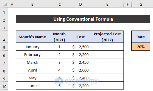
We mentioned the cost of 6 months of 2021 in the range of cells D5:D10. We considered a projection of a 20% cost increase for the following months of the next year 2022. The value of the projection rate is in cell G5.

Steps:

Select cell E5.
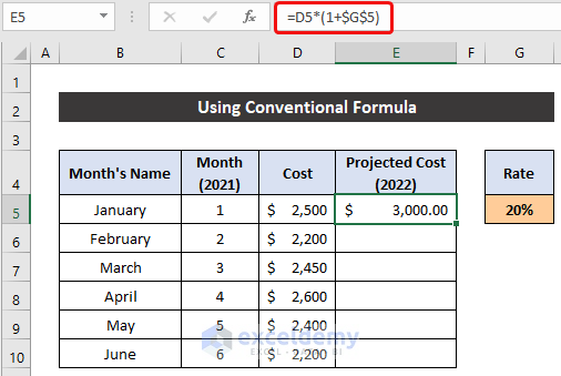
Write down the following formula into the cell. Make sure that you input the Absolute Cell Reference with cell G5.

=D5*(1+$G$5)

Press Enter.

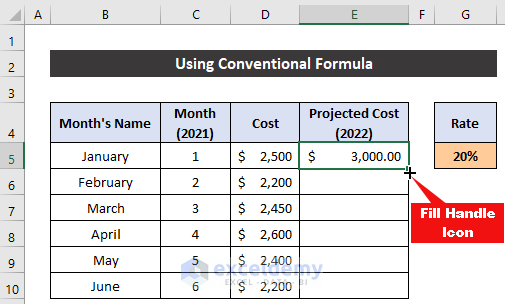
Double-click the Fill Handle icon to copy the formula up to cell E10.

Get all the projected cost values for each month.

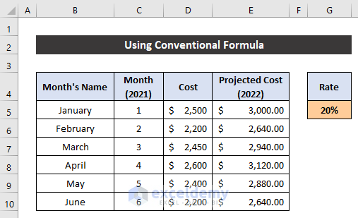
Our formula worked perfectly, and we were able to calculate the projected cost in Excel.

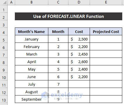
Method 2 – Use of FORECAST.LINEAR Function

The cost of the first six months is in the range of cells D5:D10. Calculate the projected cost value for the next three months of that year in the range of cell E11:E13.

Steps:

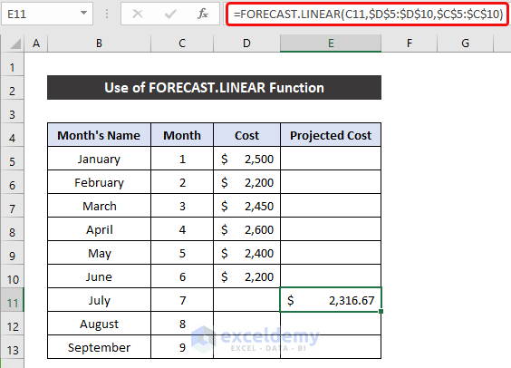
Select cell E11.
Write down the following formula into the cell to input the Absolute Cell Reference for the range of cells C5:C10 and D5:D10.

=FORECAST.LINEAR(C11,$D$5:$D$10,$C$5:$C$10)

Press Enter.

Double-click on the Fill Handle icon to copy the formula up to cell E13.
Get all the projected cost value for our desired three months.

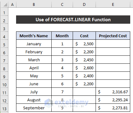
Our formula worked successfully and we can calculate the projected cost in Excel.

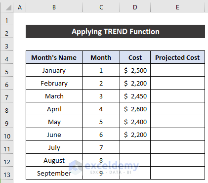
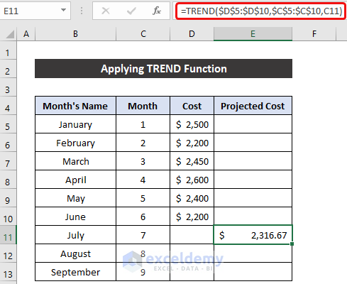
Method 3 – Applying TREND Function

The cost of the first six months is in the range of cells D5:D10 to calculate the projected cost for the next three months of that year in the range of cell E11:E13.

Steps:

Select cell E11.
Write down the following formula in the cell. Input the Absolute Cell Reference for the range of cells C5:C10 and D5:D10.

=TREND($D$5:$D$10,$C$5:$C$10,C11)

Press Enter.

Double-click the Fill Handle icon to copy the formula up to cell E13.
You will get the projected cost value for our desired three months.

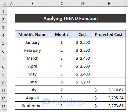
We were able to calculate the projected cost in Excel.

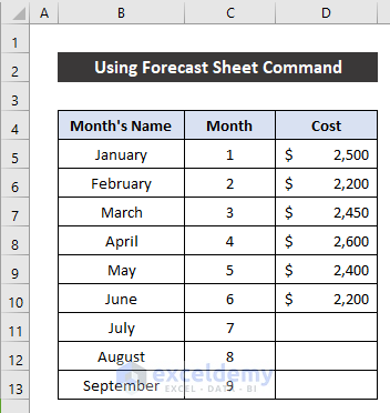
Method 4 – Using Forecast Sheet Command

This command provides us a maximum and minimum range of those projected values. In addition, this option will also supply us with a chart for understanding the data trend.

Steps:

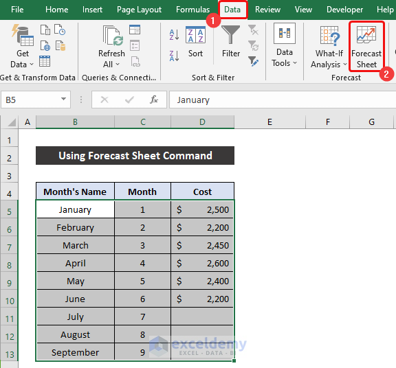
Select the range of cells B5:D13.
In the Data tab, select the Forecast Sheet option from the Forecast group.

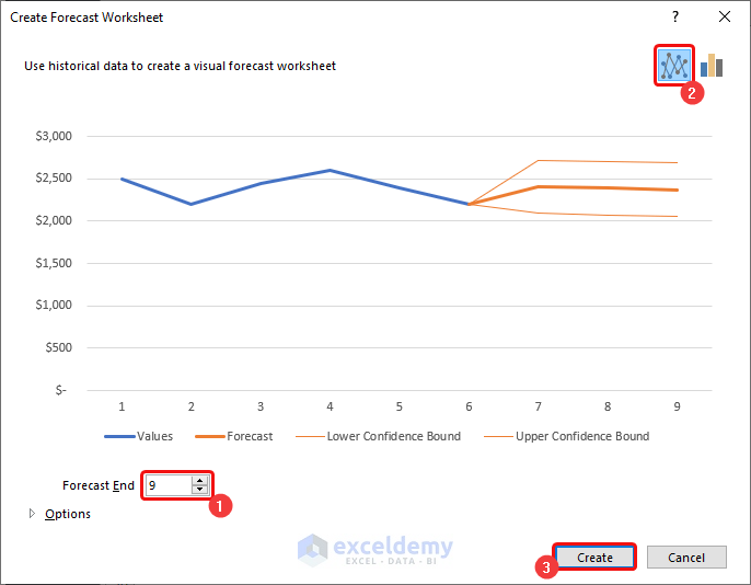
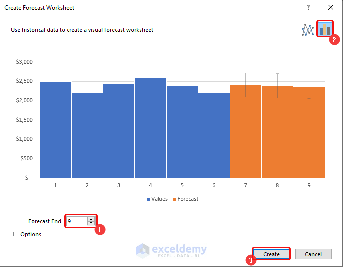
A dialog box called Create Forecast Worksheet will appear.
Set the Forecast End at 9, if the value is showing less than 9.
Choose the chart type as a line chart.
Click Create.

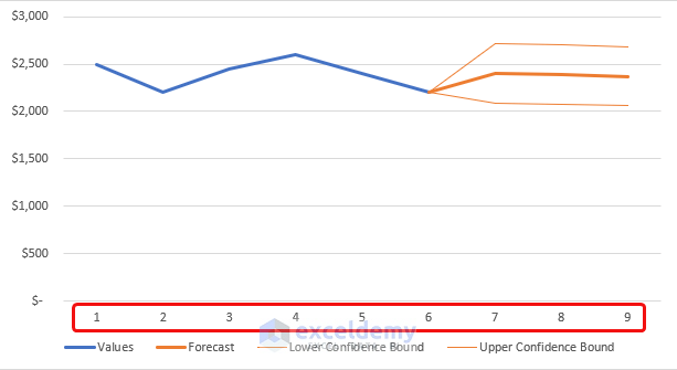
A new sheet will open with the chart and the projected values.
You may notice that the X-axis of our chart is showing the month sequence instead of the month’s names.

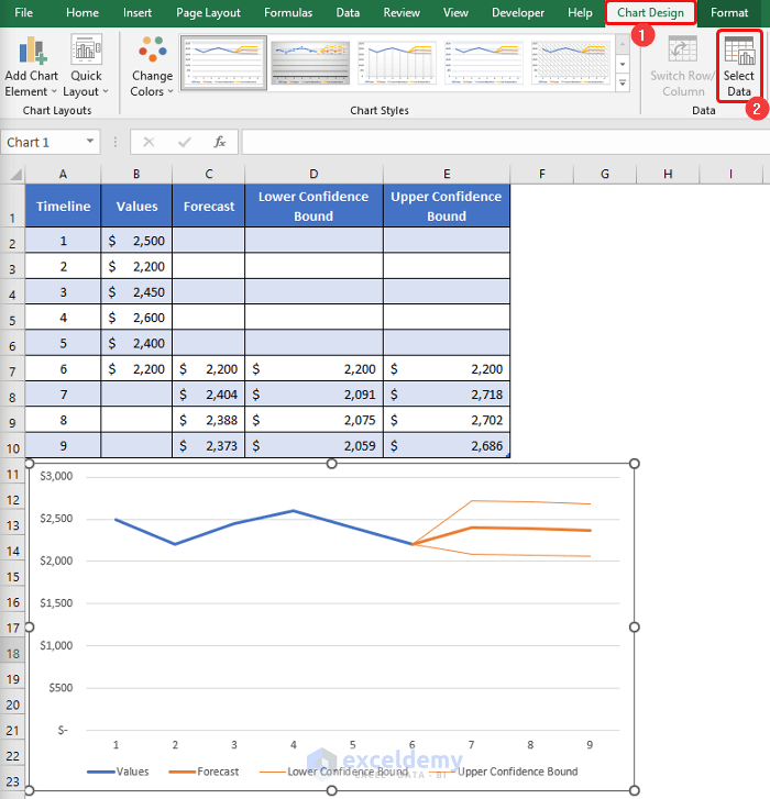
Go to the Chart Design tab and select the Select Data option.

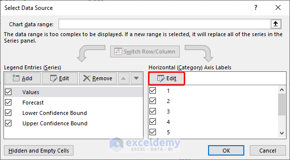
The Select Data Source dialog box will appear. Click Edit from the Horizontal (Category) Axis Labels section.

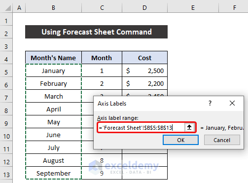
A dialog box entitled Axis Labels will appear.
Select the range of cells B5:B13 from the sheet titled Forecast Sheet and click OK.

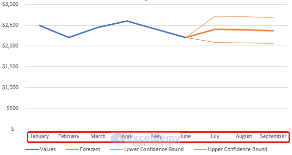
Press OK to close the Select Data Source dialog box. You will see the month’s name will appear on the X-axis.

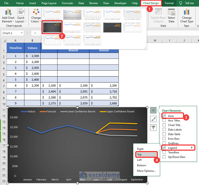
You can also modify the chart style from the Chart Design and Format ribbon.
We chose Style 6 from the Chart Styles group.
Select the Chart Elements icon and check the Axes and Legend at the Top option.

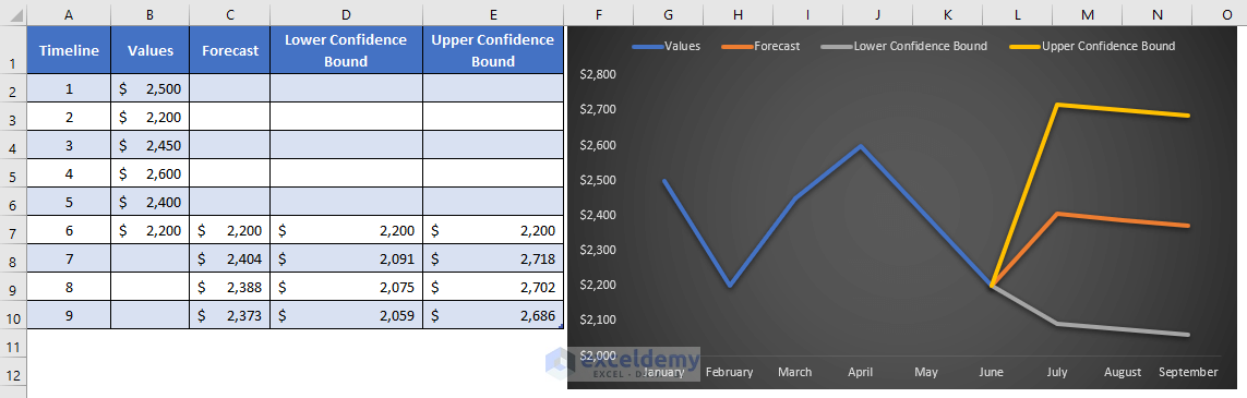
To visualize the data changing pattern more precisely, we reduced the lower boundary of the Y-axis of our chart. Double-click on the values of the Y-axis.
A side window called Format Axis will appear.
Click the drop-down arrow of the Axis Options and go to the Axis Options tab.
Set the Minimum bound as 2000 and press Enter. The class intervals in the Y-axis below 2000 will disappear and the data pattern will show in a large view.

The task for this chart is completed.

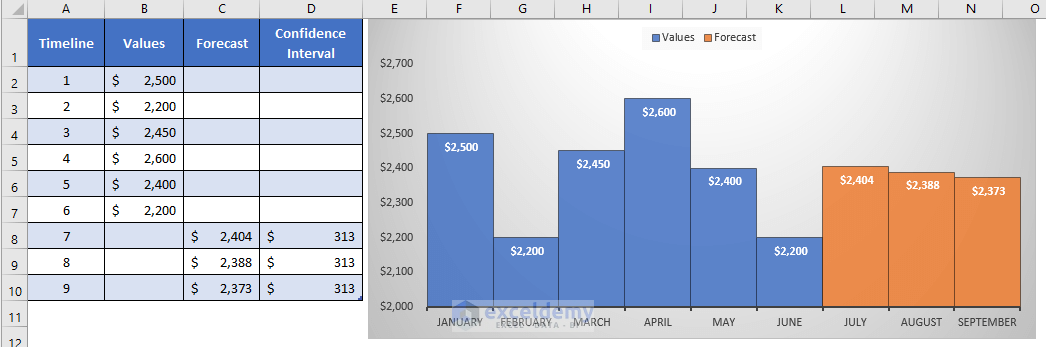
Add a column chat from the Create Forecast Worksheet dialog box. You won’t get the upper and lower projected cost range.
Choose Column Chart.