Absolute Cell Reference Shortcut in Excel – 4 Examples

Absolute cell reference is necessary when we want to lock the position of a cell in order to copy it for further use.

This is an the overview.

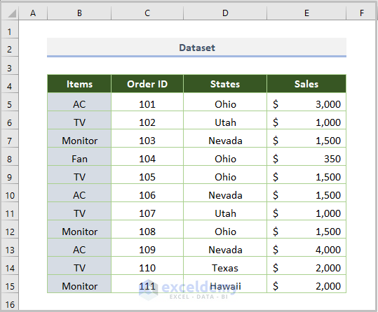
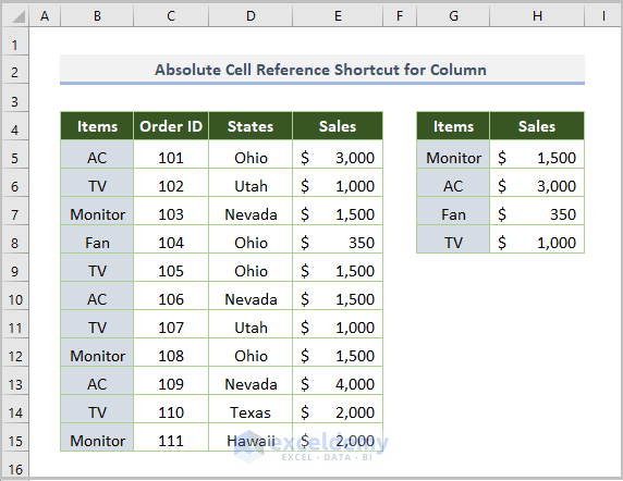
The following dataset showcases items, their order ID, states, and sales.

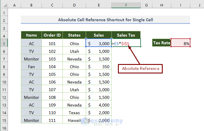
Example 1 – Absolute Cell Reference Shortcut for a Single Cell

The tax rate in percentage is given in I5. To calculate the sales tax for each item based on the tax rate and the number of sales:

Steps:

• Select the cell in which you want to calculate the sales tax
• Press the Equal (=) sign and enter the following formula.

E5 is the first cell in sales and $I$5 is the tax rate

• Move the cursor to I5 and press F4 once. You’ll see the absolute reference $I$5. The formula will be:

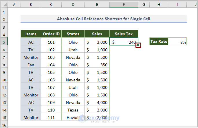
• Press Enter
• This is the output.

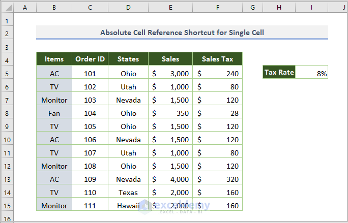
• Drag down the Fill Handle to see the result in the rest of the cells.

This is the output.

Note: In  previous versions of Excel for Mac, the shortcut of absolute cell reference is-

Related Content: What Is and How to Do Absolute Cell Reference in Excel?

Example 2 – Absolute Cell Reference Shortcut for a Cell Range

To find the. sales of ‘Monitor’ (lookup value) in B5:E15, utilize the VLOOKUP function.

Steps:

• Select the cell in which you want to see the amount of sales.
• Press the Equal (=) sign and enter the following formula.

G5 is the lookup value, B5:E15 is the table array, 4 is the column index, and FALSE is used for exact matching.

• Move the cursor to the right side of B5:E15 and press F4 once. You’ll see the absolute reference $B$5:$E$15 and the formula will be:

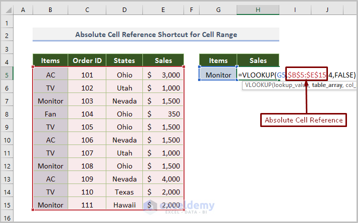
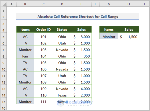
• Press Enter.
• This is the output.

Example 3 – Absolute Cell Reference Shortcut for Columns

You want to find a series of values in a column (the sales of ‘Monitor’, ‘AC’, ‘Fan’, and ‘TV’).

Steps:

• Select the cell in which you want to calculate the sales tax.
• Press the Equal (=) sign and enter the following formula.

G5 is the lookup value, B5:E15 is the table array, 4 is the column index, and FALSE is used for exact matching.

• Move the cursor to the right side G5 and press F4 thrice. You’ll see $G5 as the absolute reference. The formula will be:

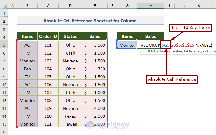
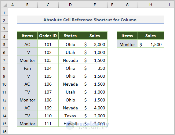
• Press Enter.
• This is the output.

• Drag down the Fill Handle to see the result in the rest of the cells.
• This is the output.

Example 4 – Absolute Cell Reference Shortcut for Rows

To find a series of values in a row:

Steps:

• Select the cell in which you want to calculate the sales tax.
• Press the Equal (=) sign and enter the following formula.

H5 is the lookup value, B5:E15 is the table array, 4 is the column index, and FALSE is used for exact matching.

• Move the cursor to the right side of H5 and press F4 twice. You’ll see H$5 as the absolute reference and the formula will be:

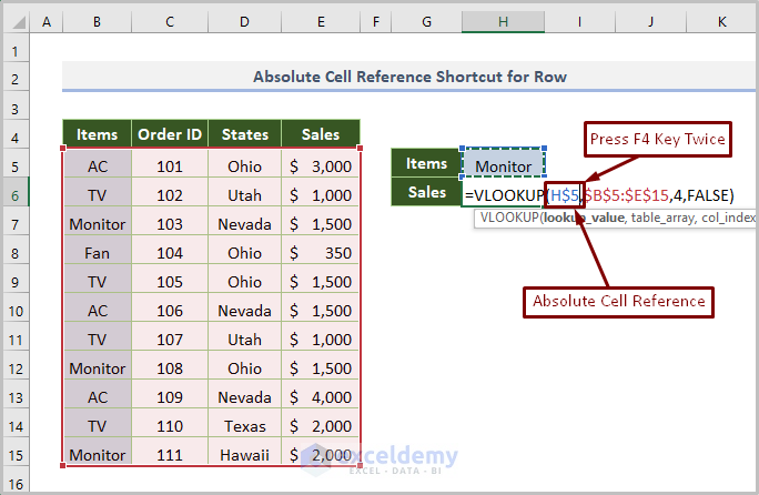
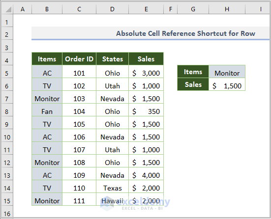
• Press Enter.
• This is the output.

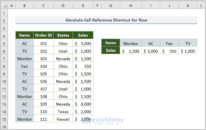
• Drag down the Fill Handle to see the result in the rest of the cells.

• This is the output.

The Shortcut Key for Absolute Reference is Not Working

Download Practice Workbook

Related Articles

• [Fixed] F4 Not Working in Absolute Cell Reference in Excel
• How to Use FormulaR1C1 Absolute Reference in Excel VBA

<< Go Back to Absolute Cell Reference | Cell Reference in Excel | Excel Formulas | Learn Excel