What Is a Discount Rate?
The discount rate is the factor used to bring future cash flows back to the present day. It also refers to the interest rate charged to commercial banks and other financial organizations for short-term loans obtained from the Federal Reserve Bank.
Method 1 – Calculate Discount Rate for Non-Compounding Interest in Excel
This method provides three ways to calculate the discount rate for non-compounding interest. Non-compounding interest (or simple interest) is computed using a loan or deposit’s principal as the base. In contrast, compounding interest considers both the principal amount and the interest accrued on it during each period. Let’s explore the procedures:
1.1 Apply Simple Formula
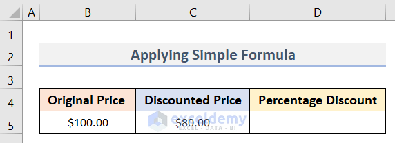
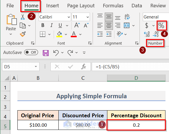
To calculate the percentage discount when you know the original price and the discounted price, follow these steps:
- In your Excel dataset (C4:D5), where you have the Original Price and the Discounted Price, divide the Discounted Price by the Original Price:
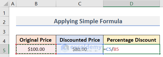
- Enter the formula below in cell D5:
=C5/B5Here, cells C5 and B5 represent the Discounted Price and the Original Price, respectively.
- After pressing Enter, you’ll get the output.
- Subtract the output from 1 using the formula in cell D5:
=1-(C5/B5)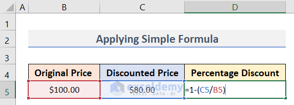
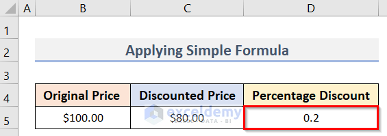
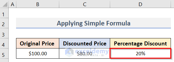
To display the result as a percentage, select cell D5, go to the Home tab, and choose the Percent Style (%) symbol.
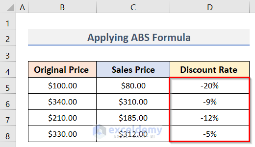
1.2 Use ABS Formula
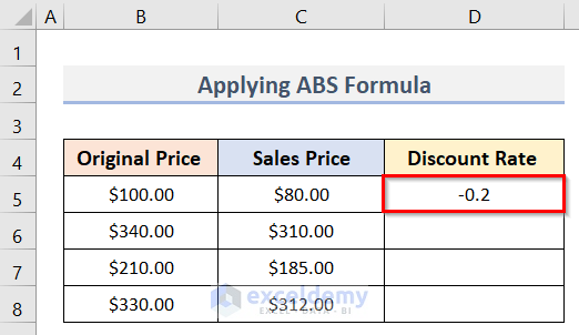
Suppose you have another dataset (B4:D8) in Excel containing Original Price and Sales Price of a Product. To calculate the Discount Rate, follow these steps:
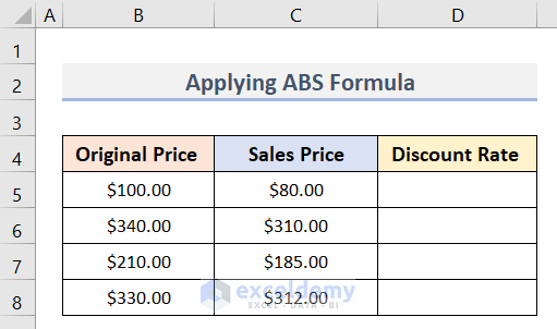
Steps:
- In the first blank cell (D5) of the Discount Rate column, enter the formula:
=(C5-B5)/ABS(B5)
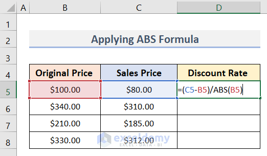
Here, cells C5 and B5 represent the Sales Price and the Original Price, respectively.
- Press Enter and get the result.
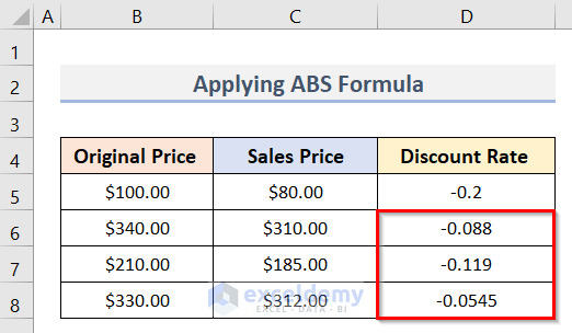
- To fill this formula into the desired range, drag the fill handle.
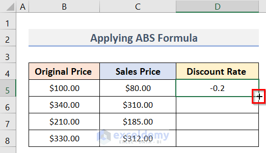
- You will get all the Discount Rate values.
- If you want the Discount Rate values in percentage form, follow the same steps as in the previous method:
- Select the range of cells (D5:D8).
- Go to the Home tab > Number group > % symbol.
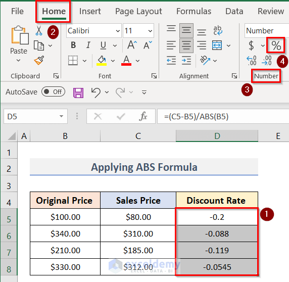
- You’ll have all the Discount Rate values. Check out the final result in the screenshot below:
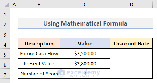
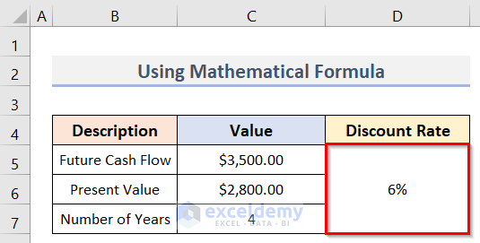
1.3 Insert Mathematical Formula
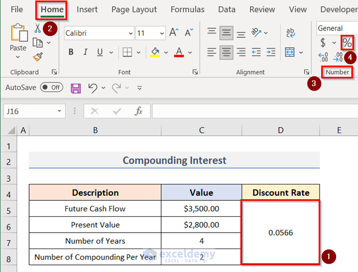
Let’s consider a dataset (B4:D7) in Excel containing Future Cash Flow, Present Value, and Number of Years. Our goal is to determine the value of the Discount Rate using a mathematical formula. Follow these steps:
- Calculate the Discount Rate:
- Select the blank cell below the “Discount Rate” heading.
- Enter the formula:
=((C5/C6)^(1/C7))-1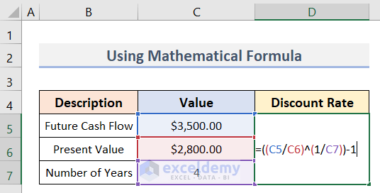
In the formula:
-
-
- C5: Future Cash Flow
- C6: Present Value
- C7: Number of Years
-
-
- Press Enter to obtain the Discount Rate value.
- Display as Percentage:
- Select the cell with the Discount Rate value.
- Go to the Home tab, select the Number group and click on % symbol.
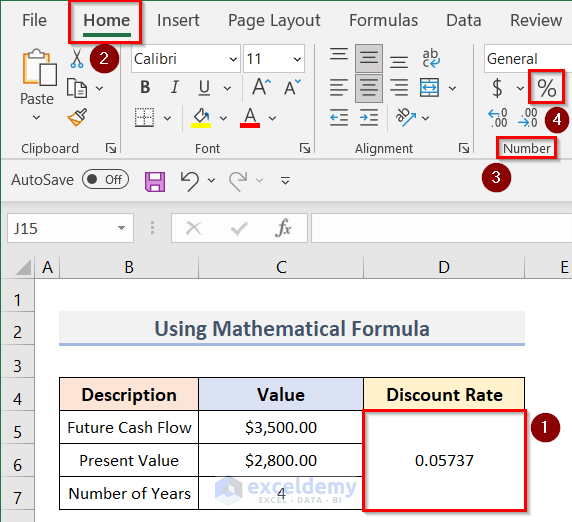
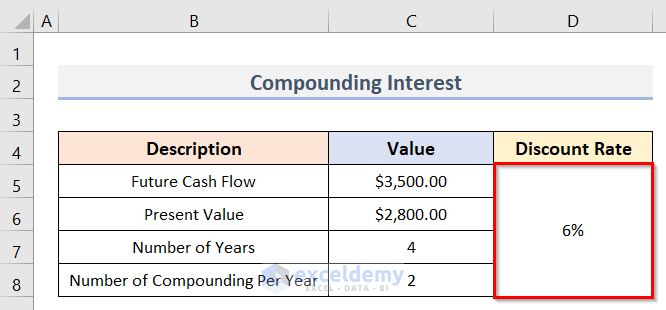
- The final result is shown in the screenshot below:
Method 2 – Determine Discount Rate for Compounding Interest
Let’s explore how compounding affects the discount rate. Suppose we have another dataset (B4:D8) in Excel with values for Future Cash Flow, Present Value, Number of Years, and Number of Compounding Per Year. Follow these steps:
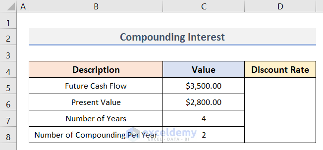
- Calculate the Discount Rate:
- Select the cell where you want to display the Discount Rate.
- Enter the formula:
=C8*((C5/C6)^(1/(C8*C7))-1)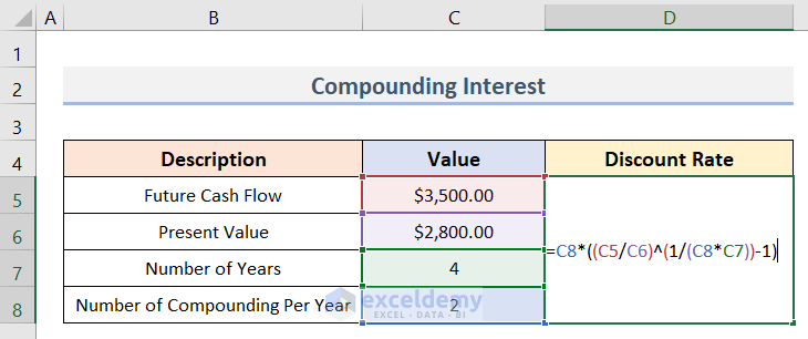
In the formula:
-
-
- C5: Future Cash Flow
- C6: Present Value
- C7: Number of Years
- C8: Number of Compounding Per Year
-
-
- Press Enter to obtain the result.
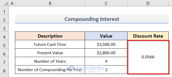
- Convert to Percentage:
- Follow the same steps as in the previous methods:
- Select the cell with the Discount Rate value.
- Go to the Home tab, select the Number group and click on % symbol.
- Follow the same steps as in the previous methods:
- The final result will be similar to the screenshot below.
Method 3 – Calculate Discount Rate for NPV in Excel
The Net Present Value (NPV) represents the value of all future cash flows, both positive and negative, discounted to the present. In this method, we’ll explore two ways to calculate the Discount Rate for NPV.
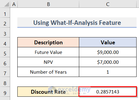
3.1 Use Excel What-If-Analysis Feature
To determine the Discount Rate for NPV, we can leverage Excel’s What-If Analysis feature. Follow these steps:
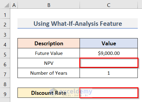
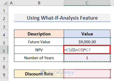
- Input NPV:
- Select cell C6 and enter the formula:
=C5/(1+C9)^C7Here:
-
-
- C5: Future Value
- C6: NPV
- C7: Number of Years
- C9: Discount Rate (initially absent)
-
-
- Press Enter.
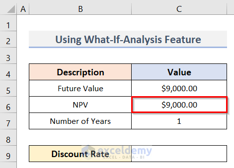
-
- Excel will compute an NPV of $9,000 (due to the absence of an interest rate), but we’ll disregard this value.
- Goal Seek:
- Select cell C9.
- Go to the Data tab, select Forecast, click on the What-If Analysis dropdown and choose Goal Seek.
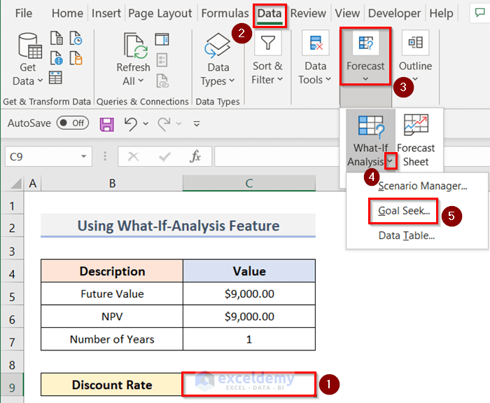
-
- Set C6 to $7,000 (our desired NPV) by adjusting the Discount Rate (C9).
- Click OK.
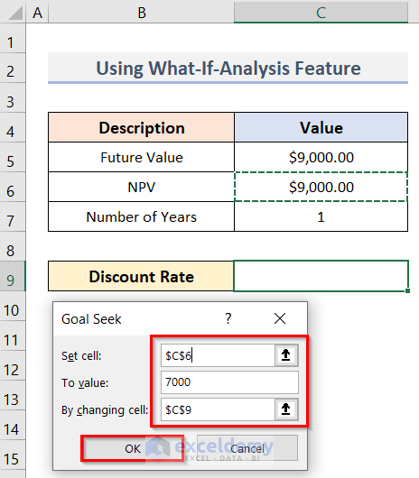
- In the Goal Seek Status window, click OK again.
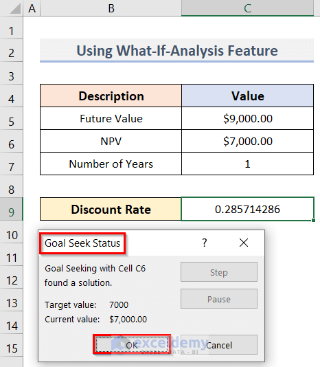
- Excel will calculate the required Discount Rate to achieve an NPV of $7,000.
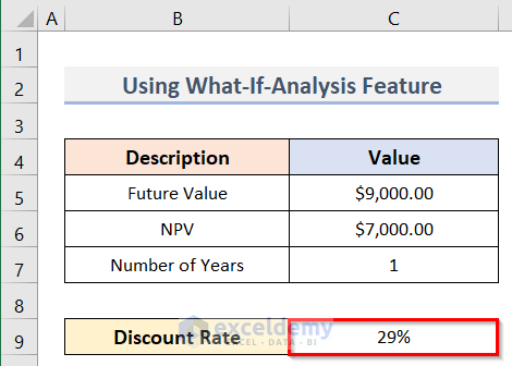
- Display as Percentage:
- Select cell C9.
- Go to the Home tab, select the Number group and click on % symbol.
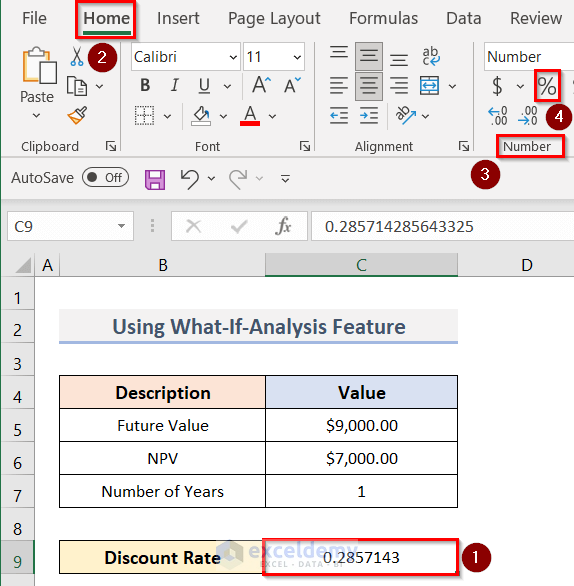
- The final result is shown in the screenshot below:
3.2 Applying Excel’s RATE Function
The RATE function is useful when dealing with a sequence of cash flows. Let’s consider an example:
Suppose you borrowed $30,000 from a bank today and need to repay it over 5 years. You’ll pay $12,000 annually. To calculate the Discount Rate, follow these steps:
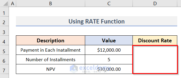
- Calculate the Discount Rate:
- Select a blank cell and enter the formula:
=RATE(C6,-C5,C7)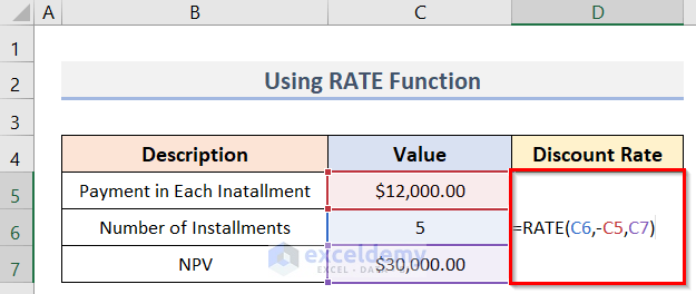
Note:
- The first argument, nper, states that there will be 5 installments.
- The following one is pmt, which displays the cash flow for every installment. A minus sign (–) is there before C5 as you can see. That is because you are paying that amount.
- The net present value, or pv, is the following argument.
- Press Enter to get the result.
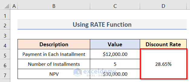
- According to this calculation, you’re paying a 28.65% discount rate on the loan.
Things to Keep in Mind
The payment (pmt) should be negative when using the RATE function.
Download Practice Workbook
You can download the practice workbook from here:
<< Go Back to Discount | Formula List | Learn Excel
Get FREE Advanced Excel Exercises with Solutions!
