What is a Financial Statement?
Financial statements, also known as financial reports, are summary documentation of the financial condition of an organization, summarizing a company’s performance throughout the year.
How to Automate Financial Statements in Excel: with Easy Steps
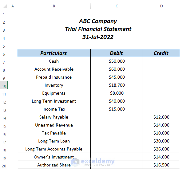
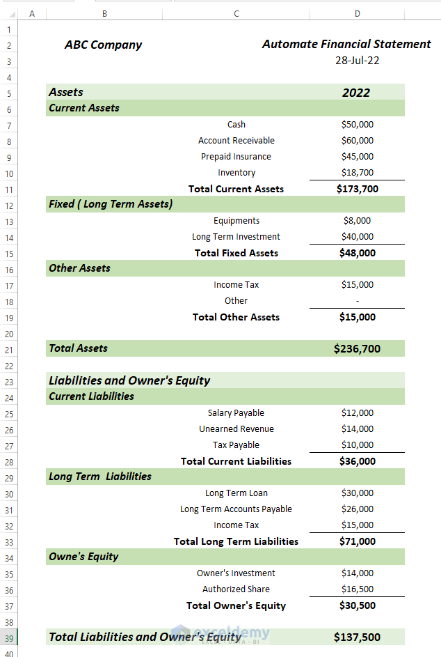
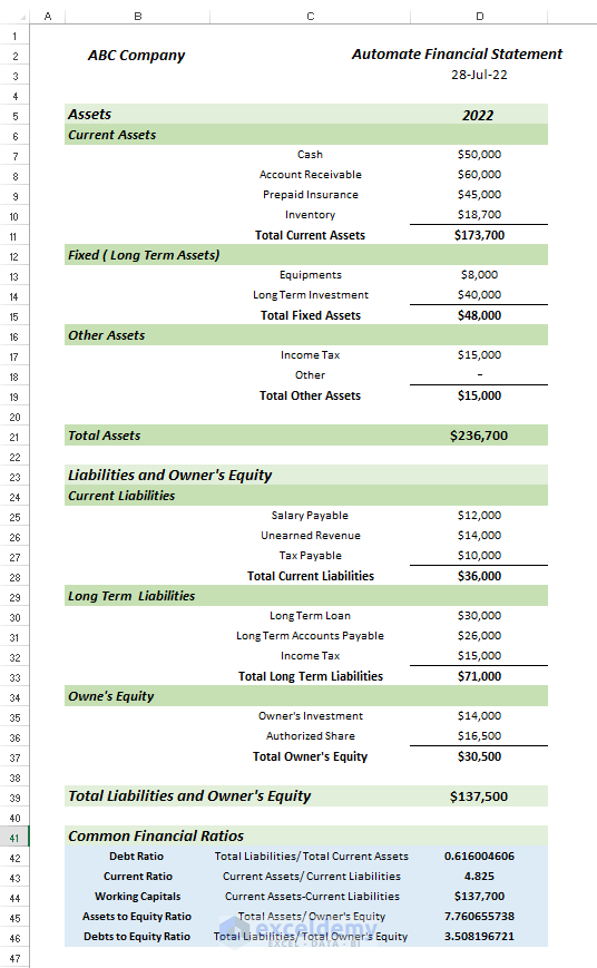
The following picture shows a Trial Financial Statement of ABC company. Using this Trial Financial Statement, we will demonstrate how to automate financial statements in Excel. We used Microsoft Office 365, but you can use any available Excel version.
Step 1 – Calculating Total Current Assets
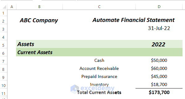
In a Financial Statement, Assets are a combination of Current Assets, Fixed ( Long Term Assets), and Other Assets.
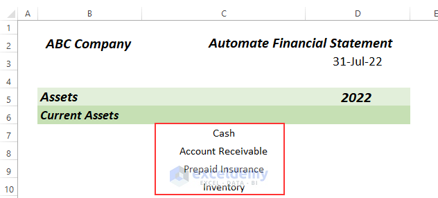
To begin, we calculate the total Current Assets. From the Trial Financial Statement, the current assets are Cash, Account Receivable, Prepaid Insurance, and Inventory.
- In the Trial Financial Statement, add entries in cells C7:C10 for Cash, Account Receivable, Prepaid Insurance, and Inventory in the Current Assets group.
- If you have more current assets in your Trial Financial Statement, include them in the Current Assets group too.
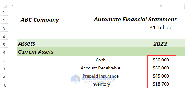
- In cells D7:D10, insert the values of the Current Assets from the Trial Financial Statement.
Now we’ll use the SUM function to calculate the Total Current Assets.
- Enter the following formula in cell D11:
=SUM(D7:D10)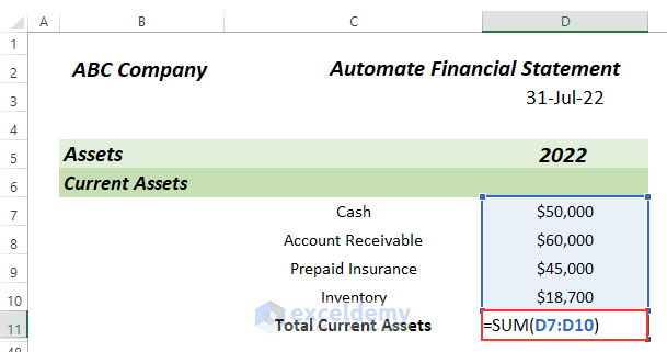
- Press ENTER.
Total Current Assets are returned in cell D11.
Read More: How to Prepare Financial Statements from Trial Balance in Excel
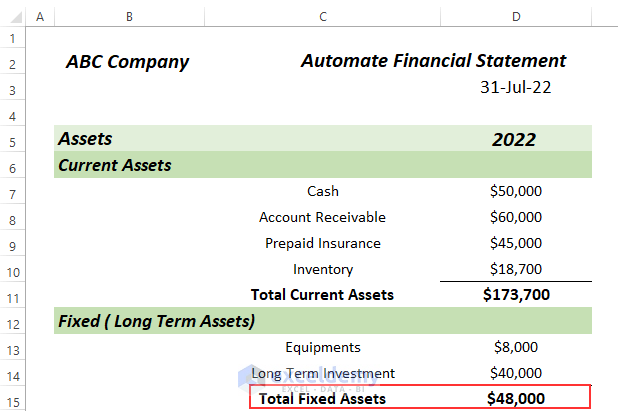
Step 2 – Computing Total Fixed Assets
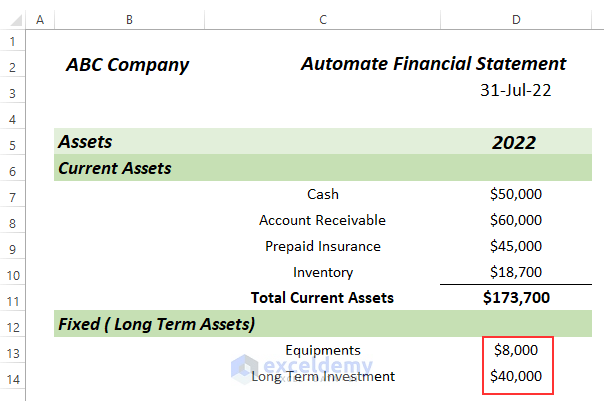
Next we calculate the Total Fixed Assets, also known as long-term assets. From the Trial Financial Statement, we identify Equipment and Long Term Investment as Fixed Assets, and calculate the Total Fixed Assets.
- Insert Equipment and Long Term Investment in the Fixed ( Long Term Assets) group in cells C13:C14.
- If you have more fixed assets in your trial Financial Statement, include them in this group.
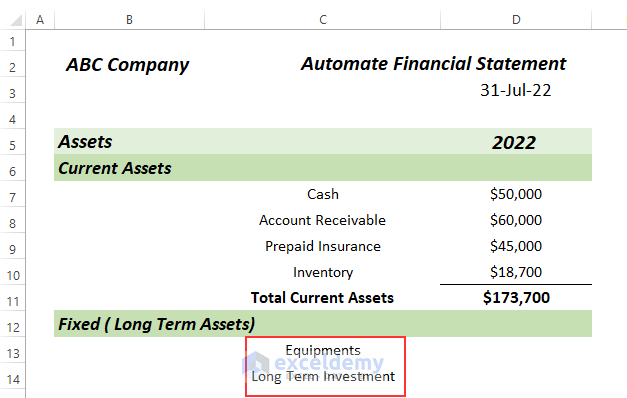
- In cells D13:D14, insert the values of Fixed Assets from the Trial Financial Statement.
We again use the SUM function to calculate the Total Fixed Assets.
- Enter the following formula in cell D15:
=SUM(D13:D14)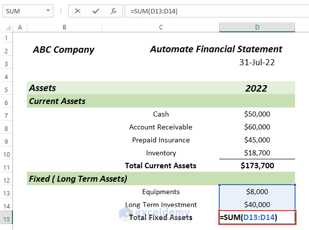
- Press ENTER.
Total Fixed Assets are shown in cell D15.
Read More: How to Create a Personal Financial Statement in Excel
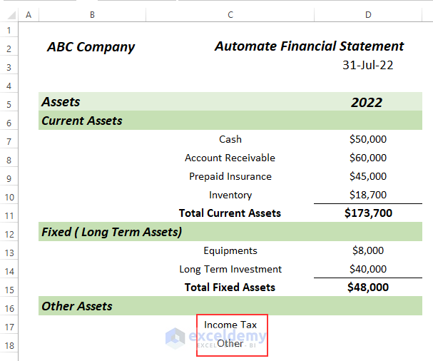
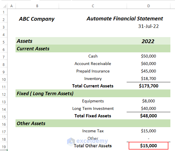
Step 3 – Finding Other Assets
Next, we calculate the Total Other Assets.
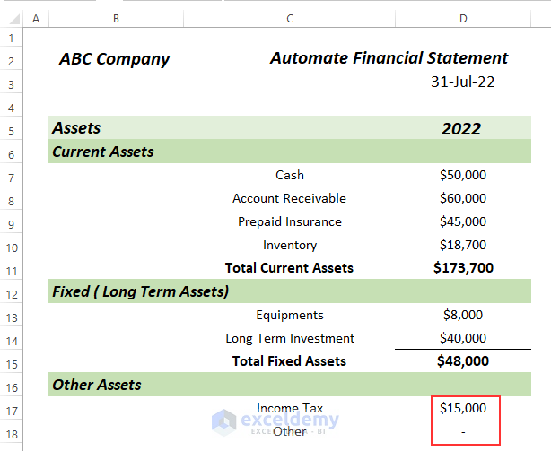
- From the Trial Financial Statement, insert Income Tax in the Other Assets group in cell C17.
- Enter Other in cell C18, in case in the future there more assets that need to be included under Other Assets.
- In cell D17, insert the value of Income Tax from the Trial Financial Statement.
- Enter the following formula in cell D19 to calculate Total Other Assets:
=SUM(D17:D18)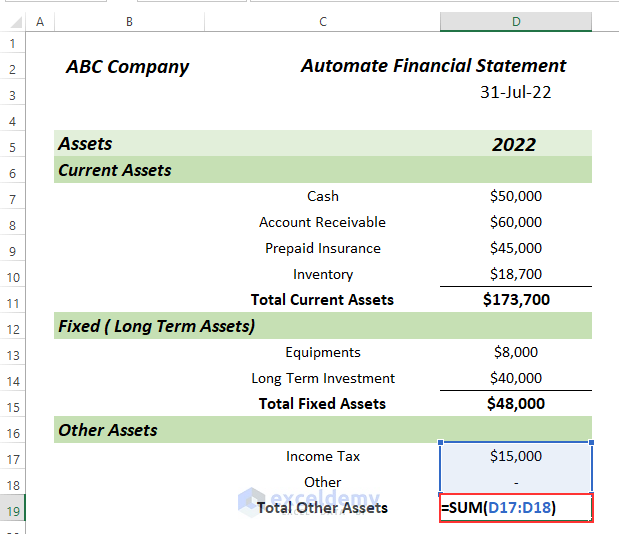
- Press ENTER.
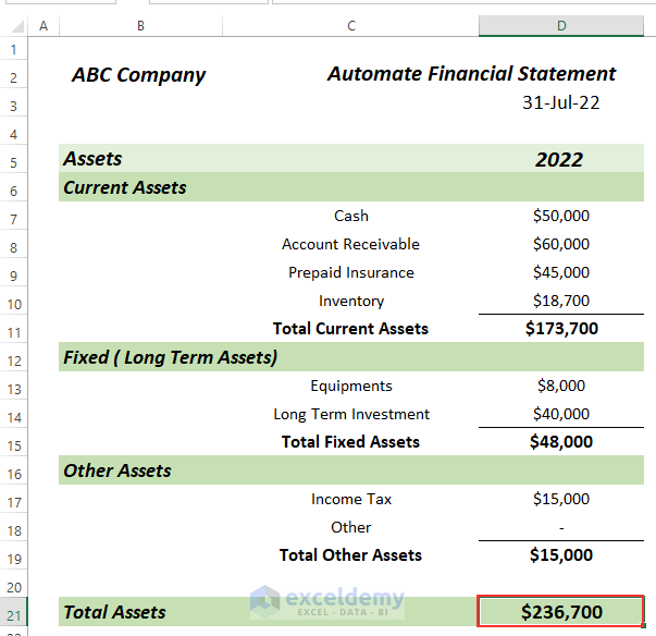
Step 4 – Determining Total Assets
- Enter the following formula in cell D21:
=D11+D15+D19This simply adds Total Current Assets, Total Fixed Assets, and Total Other Assets.
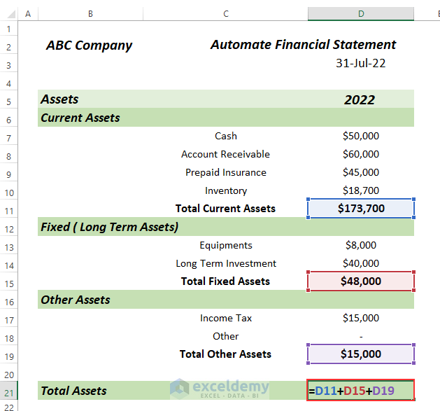
- Press ENTER.
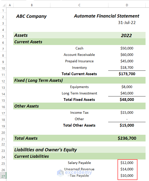
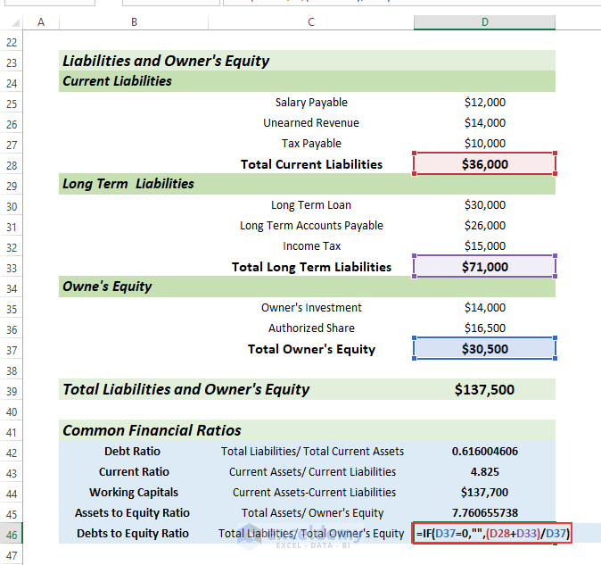
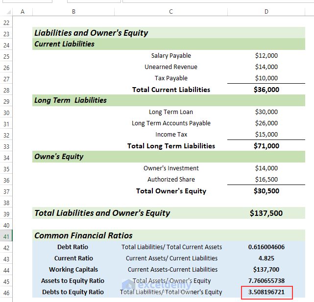
Step 5 – Calculating Total Current Liabilities
Liabilities and Owner’s Equity is a combination of Current Liabilities, Long Term Liabilities, and Owner’s Equity.
First we calculate the total Current Liabilities.
- From the Trial Financial Statement, insert Salary Payable, Unearned Revenue, and Tax Payable in the Current Liabilities group in cells C25:C27.
- If you have more Current Liabilities, include them in this group.
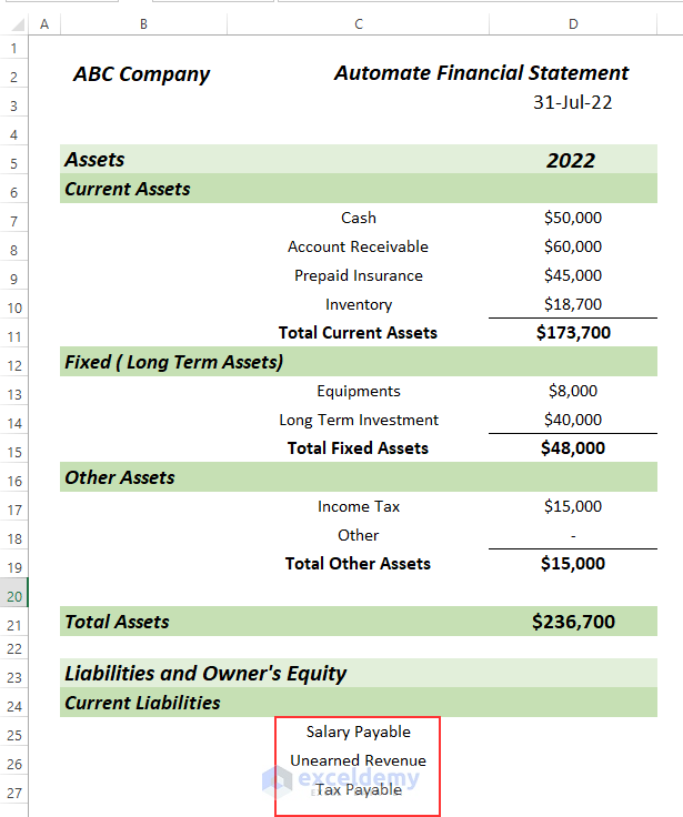
- In cells D25:D27, insert the values of Current Liabilities from the Trial Financial Statement.
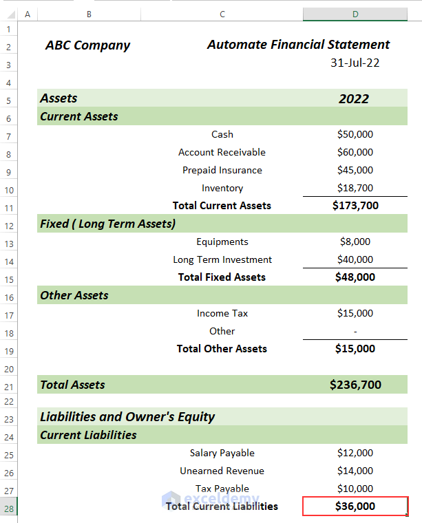
- Enter the following formula in cell D28 to calculate the Total Current Liabilities:
=SUM(D25:D27)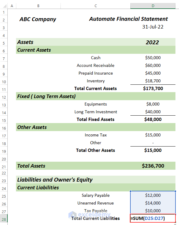
- Press ENTER.
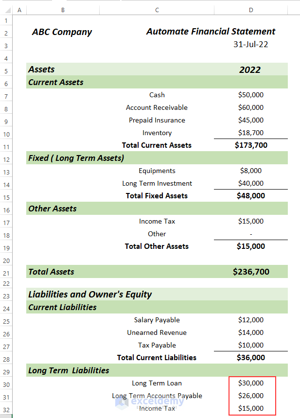
Step 6 – Computing Total Long Term Liabilities
- From the Trial Financial Statement, insert Long Term Loan, Long Term Account Payable, and Income Tax in the Long Term Liabilities group.
- If you have more Long Term Liabilities, include them in this group.
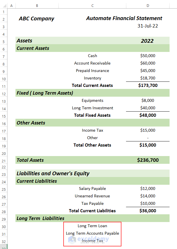
- In cells D30:D32, insert the values of Long Term Liabilities from the Trial Financial Statement.
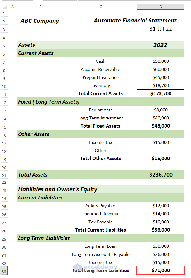
- Enter the following formula in cell D33 to calculate the Total Long Term Liabilities:
=SUM(D30:D32)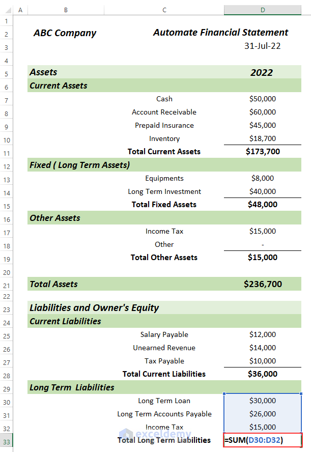
- Press ENTER.
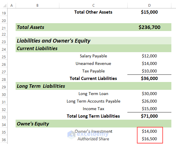
Step 7 – Finding Total Owner’s Equity
- From the Trial Financial Statement, insert the Owner’s Investment and Authorized Share in the Owner’s Equity group.
- If you have more Owner’s Equity categories, include them in this group.
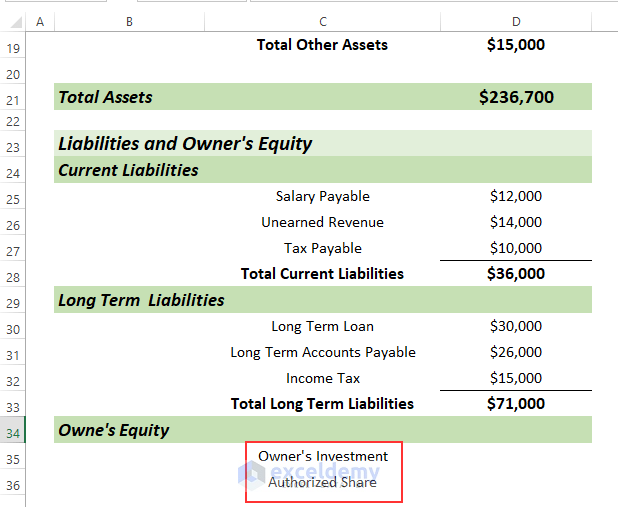
- In cells D35:D36, insert the values of Owner’s Equity from the Trial Financial Statement.
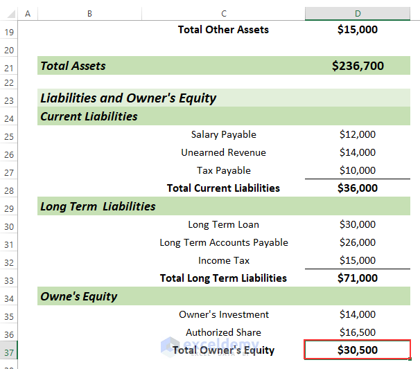
- Enter the following formula in cell D37 to calculate the Total Long Term Liabilities:
=SUM(D35:D36)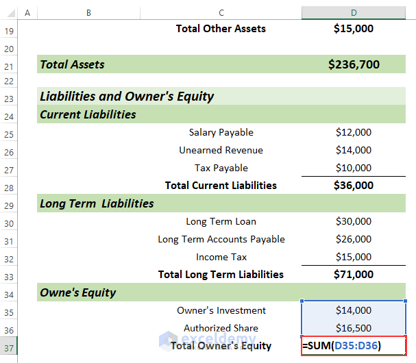
- Press ENTER.
Step 8 – Determining Total Liabilities and Owner’s Equity
- Enter the following formula in cell D39:
=D28+D33+D37This simply adds Total Current Liabilities, Total Long Term Liabilities, and Total Owner’s Equity.
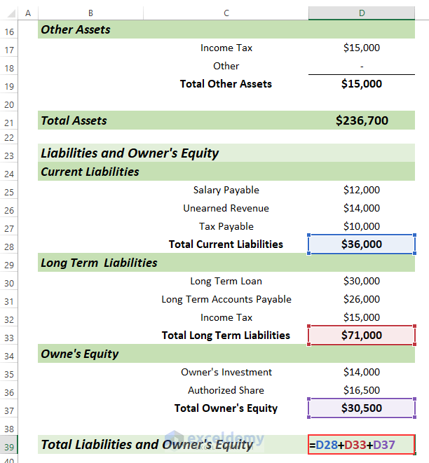
- Press ENTER.
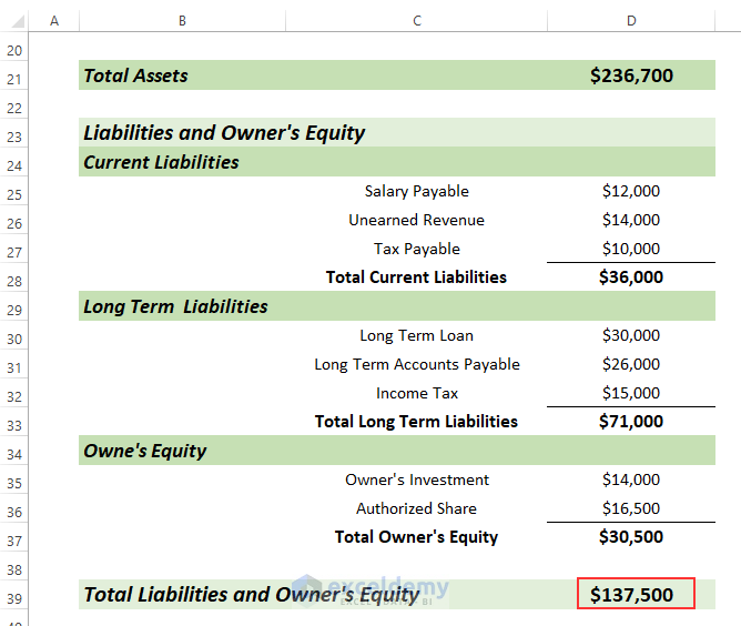
Our automated financial statement is complete.
Read More: How to Link 3 Financial Statements in Excel
Calculating Common Financial Ratios in Financial Statements
Financial statements contain several financial ratios, which give an overall view of the financial statements. Let’s determine the common financial ratios.
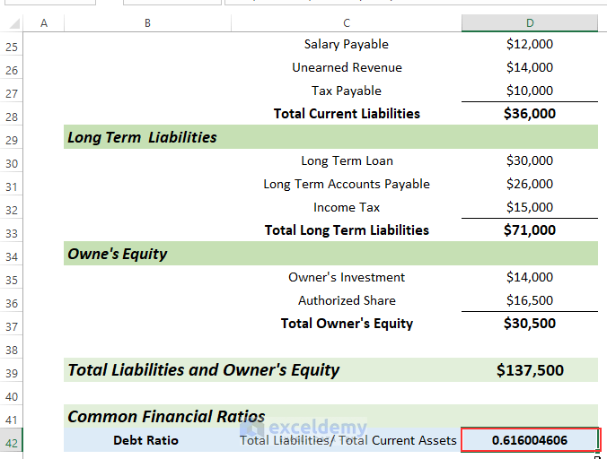
Step 1 – Calculating the Debt Ratio
Debt Ratio = Total Liabilities/ Total Current Assets
- Enter the following formula in cell D42:
=IF(D11=0,"",(D28+D33)/D11)
Formula Breakdown
- IF(D11=0,””,(D28+D33)/D11) → the IF function returns a blank cell when D11 is 0, otherwise it returns the value of the division.
- (D28+D33) → are the Total Liabilities.
- D11 → is the Total Current Assets.
- IF(D11=0,””,(D28+D33)/D11) → becomes
- Output: 0.616004606
- Explanation: as D11 is not equal to 0, the IF function returns the value of the division. 616004606 is the debt ratio.
- Press ENTER.
The Debt Ratio is returned in cell D42.
Read More: Consolidation of Financial Statements in Excel
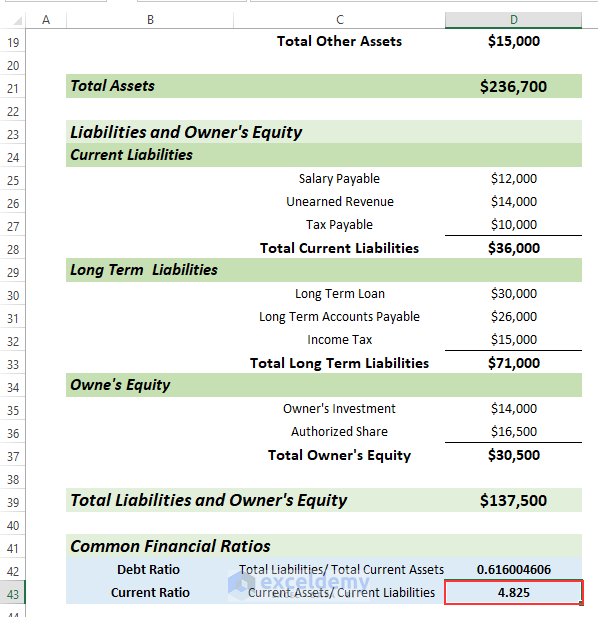
Step 2 – Computing the Current Ratio
Current Ratio = Current Assets/ Current Liabilities
- Enter the following formula in cell D43:
=IF(D28=0,"",D11/D28)Here, the IF function returns a blank cell when D28 is 0, otherwise it returns the value of the division.
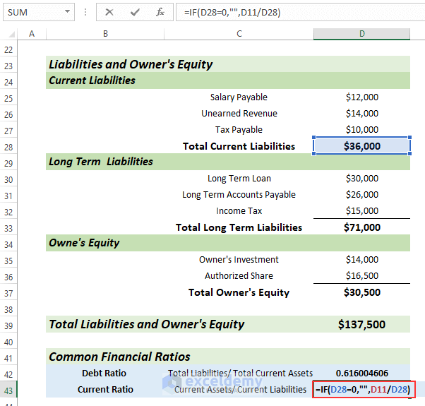
- Press ENTER.
The Current Ratio is returned in cell D43.
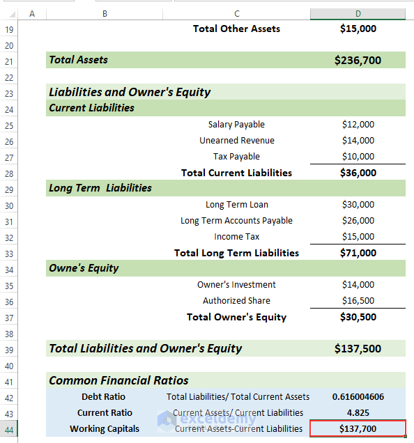
Step 3 – Finding the Working Capital
Working Capital = Current Assets-Current Liabilities
- Enter the following formula in cell D44:
=D11-D28This simply subtracts cell D28 from cell D11.
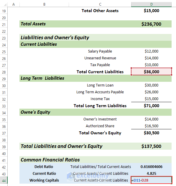
- Press ENTER.
Working Capital is returned in cell D44.
Step 4 – Determining the Assets to Equity Ratio
Assets to Equity Ratio = Total Assets/Total Owner’s Equity
- Enter the following formula in cell D45:
=IF(D37=0,"",D21/D37)Here, the IF function returns a blank cell when D37 is 0, otherwise it returns the value of the division.
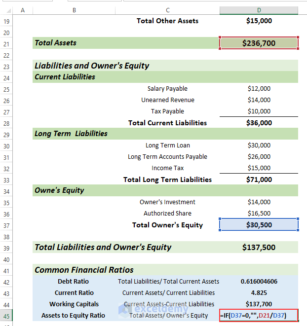
- Press ENTER.
The Assets to Equity Ratio is returned in cell D45.
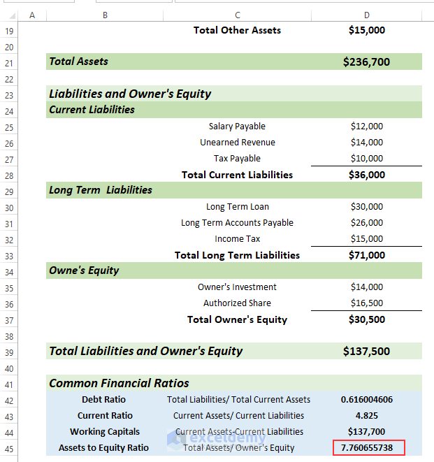
Step 5 – Calculating Debts to Equity Ratio
Debts to Equity Ratio = Total Liabilities/Total Owner’s Equity
- Enter the following formula in cell D46:
=IF(D37=0,"",(D28+D33)/D37)Here, the IF function returns a blank cell when D37 is 0, otherwise it returns the value of the division.
- Press ENTER.
The Debts to Equity Ratio is returned in cell D45.
The automated financial statement with common financial ratios is complete.
Download Practice Workbook
You can download the Excel file and practice while you are reading this article.
Related Articles
<< Go Back to How to Create Financial Statements in Excel | Excel for Finance | Learn Excel
Get FREE Advanced Excel Exercises with Solutions!
