How to Subtract and Display Negative Time in Excel? -

If you are working with the time or date format in Excel and if you subtract a time value from another, then there is a possibility that you will come across a negative time value. If the cell contains a negative time or date value then Excel might show ##### instead of the correct format of the value. In this tutorial, I will show you how to subtract and display negative times in Excel.

How to Subtract and Display Negative Time in Excel – 3 Methods

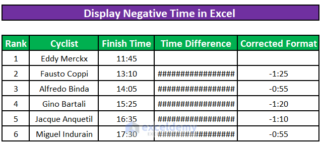
Suppose you have an Excel file that contains information about the time 6 cyclists took to complete a cycling contest. Cyclists were ranked in ascending order. The sheet has the Rank, Cyclist’s name, Finish Time, Time Difference between two successive cyclists, and the Corrected Format to show the negative time after subtraction.

Method 1 – Use the 1904 Date System to Subtract and Display Negative Time in Excel

Step 1:

⦿ Click the File tab.

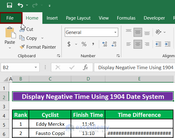
⦿ Click Options.

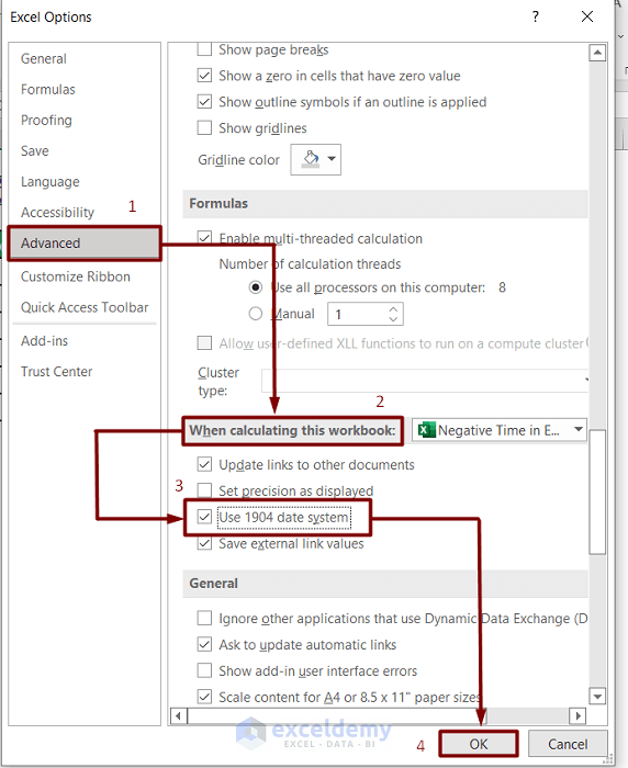
Step 2:

⦿ Click Advanced options on the left pane.

⦿ Scroll down the displayed window and choose When calculating this workbook. Tick Use 1904 date system.

⦿ Click OK.

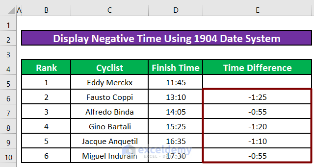
⦿ Negative times will be displayed in the correct format.

Method 2 – Apply the TEXT Function to Display Negative Time in Excel

Step 1:

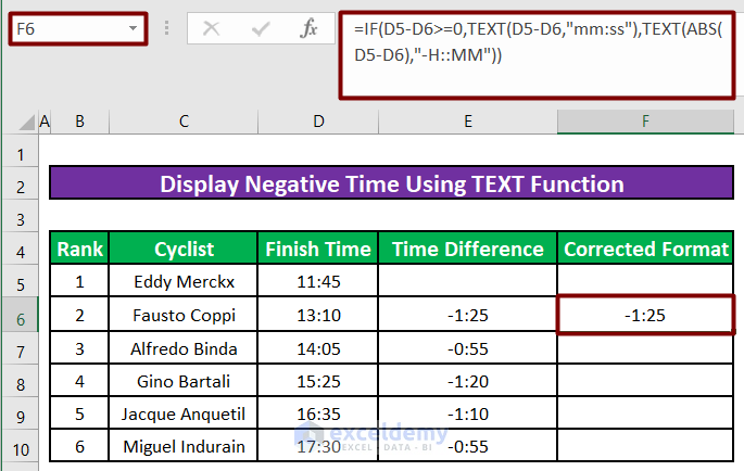
⦿ Enter the following formula in F6.

=IF(D5-D6>=0,TEXT(D5-D6,"mm:ss"),TEXT(ABS(D5-D6),"-H::MM"))

Formula Breakdown:

IF will perform a logical test (D5-D6>=0) to find out if the subtracted time value is positive. If the test returns TRUE, no changes will be made.
If the test returns FALSE, the function will first determine the absolute value of the subtracted time using the ABS feature. The TEXT feature will add a minus (-) in front of the subtracted time value using “-H::MM” as the text format.

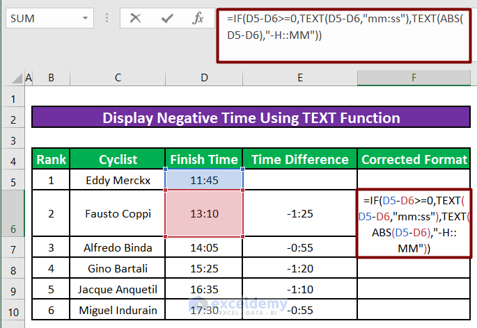
⦿ Press ENTER and negative time will be displayed in F6 in the correct format.

Step 2:

⦿ Use the Fill Handle to drag the formula across the cells you want to fill.

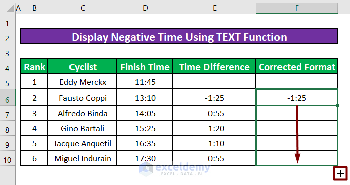
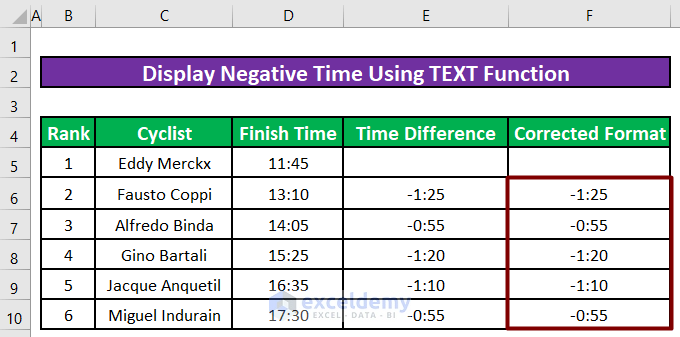
⦿ All negative times in the Corrected Format column will be displayed in the right format.

Method 3 – Using the Combination of TEXT, MAX, and MIN Formulas to Display Negative Time

Step 1:

⦿ Enter the following formula in F6.

=TEXT(MAX($D$5:$D$6)-MIN($D$5:$D$6),"-H::MM")

Formula Breakdown:

The MAX function will determine the larger value in the absolute range $D$5:$D$6 whereas the MIN function will determine the smaller one in the same range.
The smaller value in the absolute range $D$5:$D$6 will be subtracted from the larger value in that range.
The TEXT function will then put a minus (-) in front of the subtracted time value using “-H::MM” as the text format.

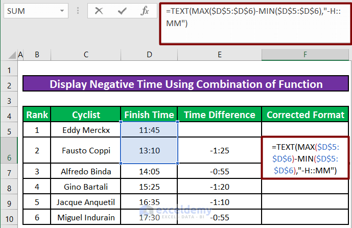
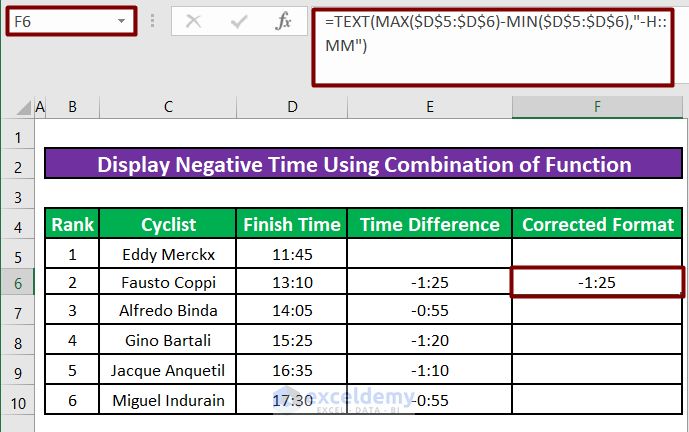
⦿ Press ENTER and negative time in F6 will be displayed in the correct format.

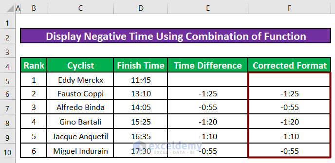
Step 2:

⦿ Enter the formula for the rest of the cells in the Corrected Format column.

Note: We cannot drag the fill handle downwards, as we are using the absolute reference ($D$5:$D$6) for the range in both MAX and MIN functions. The formula must be entered in each cell in the column.

⦿ All negative times in the Corrected Format column will be displayed in the right format.

Quick Notes

The MAX and MIN functions determine the largest and smallest values in a range. We are determining the larger and smaller values between two cells only. Therefore, cell reference must be absolute ($D$5:$D$6). Otherwise, both functions will throw errors.

Download Practice Workbook

Download this practice book to exercise the task while you are reading this article.

Negative Time in Excel.xlsx