How to Make Excel Go to Next Line Automatically (2 Examples)

We can go to the next cell in Excel easily by pressing the Enter button. But going to the next line in the same cell is not quite easy. We can do this by applying some tricks to go to the next line automatically in Excel.

How to Make Excel Go to Next Line

There is a general way to go to the next line in Excel by inserting a line break. We will add this line with a keyboard shortcut. Have a look at the method below.

📌 Steps:

We have a dataset in one sentence in a single cell.

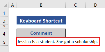
We will add a new line to the cell.

Press F2 to make the cell editable.
Move the cursor to the position of the sentence where we need a line break.

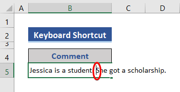
After that, press the Alt + Enter button from the keyboard.

We can see a new line added in the cell.

We can also see that Wrap Text is enabled for this cell.

Now, adjust the cell width from the row bar.

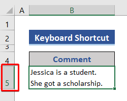
A new line was added to the cell successfully.

How to Make Excel Go to Next Line Automatically: 2 Examples

In this section, we will show 2 examples in Excel to go to the next line automatically in a cell.

1. Enable Wrap Text Feature

Wrap Text is a useful feature of Excel. In this example, we will show how we can use this feature to go to the next line within cells.

📌 Steps:

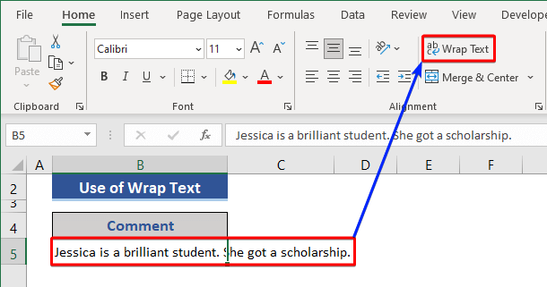
We can see there is a sentence in Cell B5.

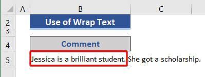
However, the width of the cell is not sufficient to accommodate the whole sentence. In this situation, we need to go to the next line to accommodate the full sentence on that cell.

Click on Cell B5.
Then, select the Warp Text feature from the Alignment group.

Look at the dataset.

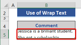
We can see a new line added in the cell.

After that, adjust the length and width of the cell by dragging the column and row or using the AutoFit feature.

Read More: How to Space Down in Excel

2. Use an Excel Formula to Join Text and Go to New Line Automatically

In this example, we will use different Excel functions to join texts first. Then we will add a new line with the joined text. We can use the ampersand, CONCATENATE, and TEXTJOIN functions to join texts. We will also use the CHAR function here. For line breaks, we use CHAR(10).

The CONCATENATE function joins several text strings into one text string.

The TEXTJOIN function concatenates a list or range of text strings using a delimiter.

📌 Steps:

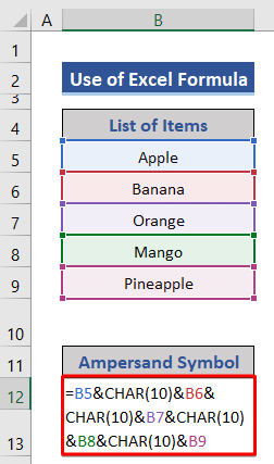
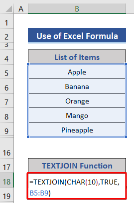
In the dataset, we have a list of fruits.

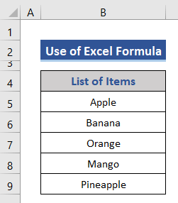
We will join those fruits and then add the new line.

We add a new row for applying a formula based on the ampersand symbol.
Enable Wrap Text for Cell B12, where we will apply the formula.

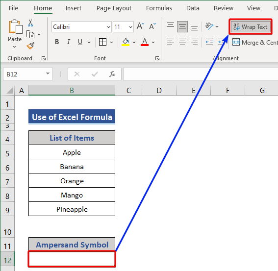
Now, insert the following formula on Cell B12 based on ampersand.

=B5&CHAR(10)&B6&CHAR(10)&B7&CHAR(10)&B8&CHAR(10)&B9

Press the Enter button.

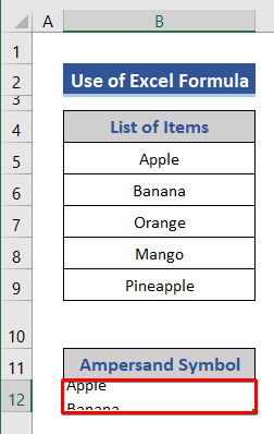
New lines are added to the cell.

Adjust the length of Cell B12.

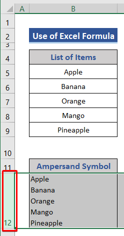
We can see new lines added successfully.

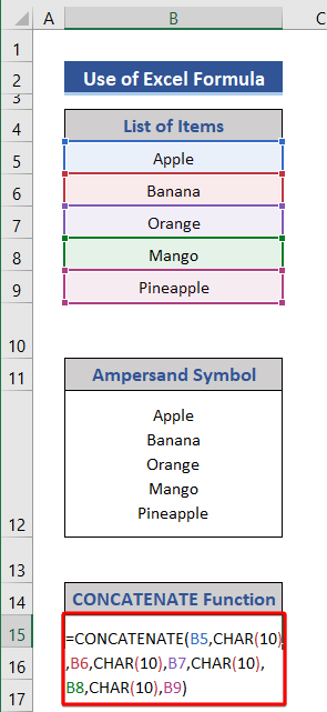
We can also use other functions in the formula to perform this task.

Put this formula based on the CONCATENATE function on Cell B15 with Wrap Text

=CONCATENATE(B5,CHAR(10),B6,CHAR(10),B7,CHAR(10),B8,CHAR(10),B9)

We can also apply a formula based on the TEXTJOIN The formula will look like this:

=TEXTJOIN(CHAR(10),TRUE,B5:B9)

After applying any of those formulas we need to adjust the length of the corresponding cell. Also, Wrap Text must be enabled for the cells.

Read More: How to Do a Line Break in Excel

How to Make Excel Go to Next Line in Formula Bar

In this example, we will show how to add a new line in a formula. Sometimes we use formulas with a larger length. To view this larger formula is not possible in a single line. There is a solution to this problem. We can introduce a new line in the formula to view easily.

📌 Steps:

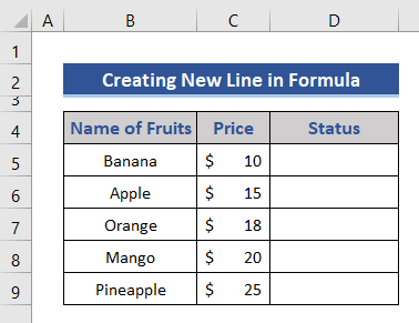
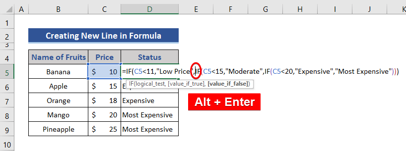
We will compare the following dataset. We will apply a formula to the Status And then add a new line in the formula.

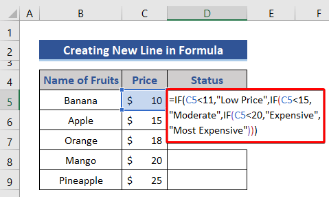
Apply the following formula to Cell D5.

=IF(C5<11,"Low Price",IF(C5<15,"Moderate",IF(C5<20,"Expensive","Most Expensive")))

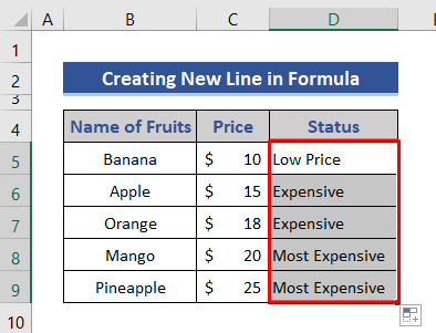
Then, press Enter and then drag the Fill Handle icon.

Now, edit the formula of Cell D5 by pressing the F2 button.
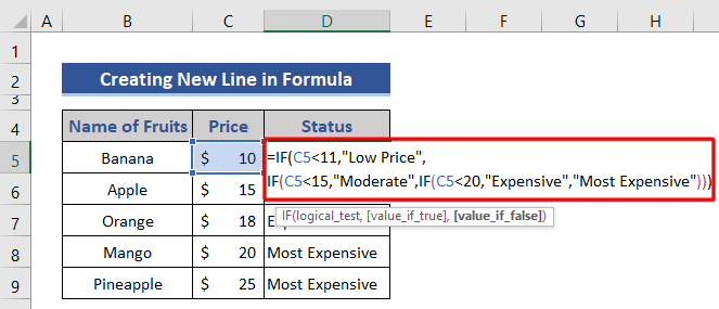
Place the cursor on the desired place. Then, press Alt + Enter.

We can see a new line is added to the formula.

Similarly, we move the cursor and add another line in the formula.

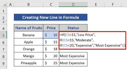
This is how we can add a new line in a formula.

How to Create New Lines After Specific Character in Excel

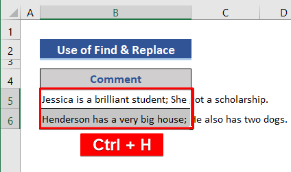
In this example, we will show how to add new lines after a specific character. We will apply the Find & Replace feature here.

📌 Steps:

We have two sentences in the dataset.

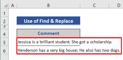
We will add a new line after the semi-colon (;).

Select Range B5:B6.
Press Ctrl + H.

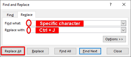
Find and Replace dialog box appears.
Input semicolon symbol (;) on Find what Because we add a new line after this character or symbol.
After that, press Ctrl + J on Replace with box.
Finally, click on the Replace All button.

We can see the number of replacements in the pop-up.

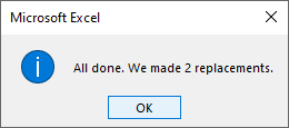
Look at the dataset.

We can see new lines inserted in the cells.

Things to Remember

Wrap Text must be enabled.
We need to adjust the cell length every time.

Download Practice Workbook

Download this practice workbook to exercise while you are reading this article.

Go to Next Line Automatically.xlsx

Conclusion

In this article, we showed how to make Excel go to the next line automatically in Excel using different examples. I hope this will satisfy your needs. Please have a look at our website and give your suggestions in the comment box.

<< Go Back to Line Break in Excel | Text Formatting | Learn Excel

Get FREE Advanced Excel Exercises with Solutions!