In today’s world, loans are an inseparable part of our lives. Sometimes, we need to use the help of loans and installments to buy our essential products. In this article, we will show you how to create an Excel loan calculator with extra payments.
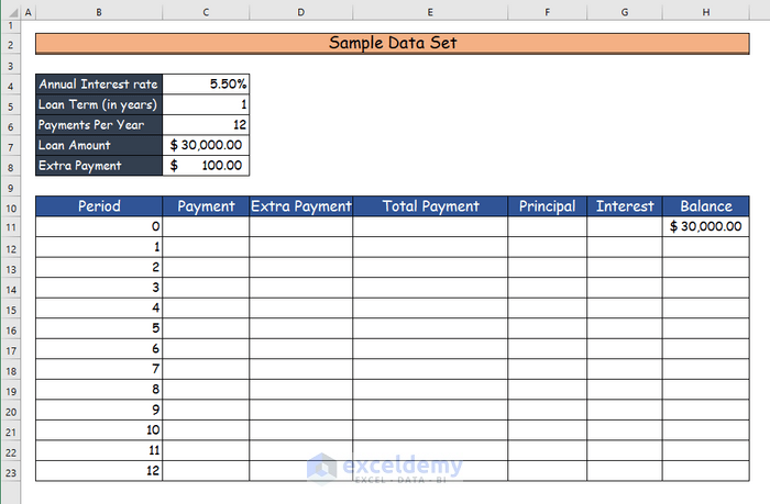
It is an important issue for the loan payer and receiver to determine and calculate the exact amount of installment or payment per month regarding the payable amount and interest rate. Using Excel in this regard will help you to determine your payable amount correctly. In loan installments, extra payments help to repay the loan earlier. In this article, we will use the IFERROR function in the first solution and a combination of the PMT, IPMT, and PPMT functions in the second approach to create an Excel loan calculator with extra payments. We will use the following sample data set to create an Excel loan calculator with extra payments.
1. Applying IFERROR Function to Create a Loan Calculator with Extra Payments in Excel
We can create an Excel loan calculator with extra payments by applying the IFERROR function.
Steps:
- Firstly, calculate the scheduled payment in cell C9.
- To do this use the following formula by applying the IFERROR function.
=IFERROR(-PMT(C4/C6, C5*C6, C7), "")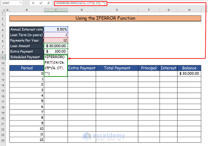
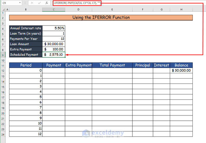
- Then, press Enter and you will get the scheduled payment in cell C9, which is $2,575.10.
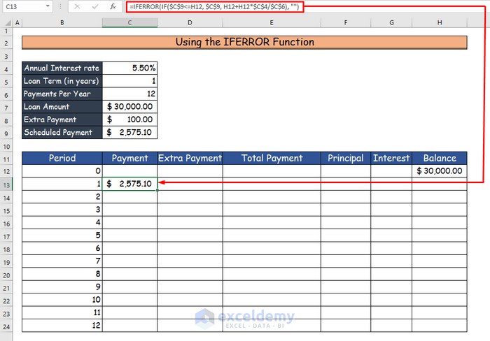
- Now, determine payment in cell C13 using the IFERROR function.
=IFERROR(IF($C$9<=H12, $C$9, H12+H12*$C$4/$C$6), "")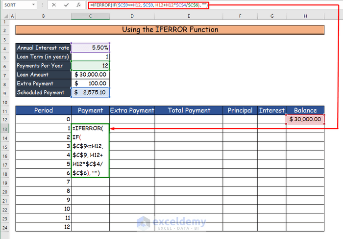
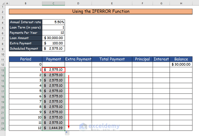
- After that, press Enter and you will get the payment for the first month in cell C13, which is $2575.10.
- Finally, AutoFill the formula down to the lower cells in column C.
- Next, determine the extra payment in column D for which you will use the IFERROR function.
=IFERROR(IF($C$8<H12-F13,$C$8, H12-F13), "")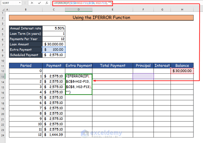
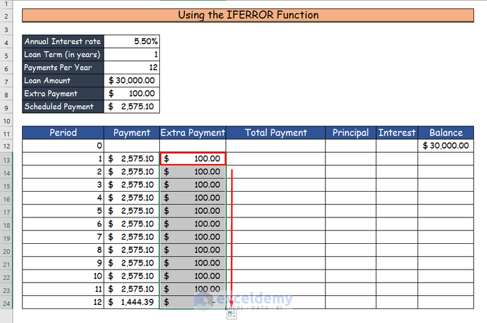
- Then, press Enter and you will get the extra payment for the first month in cell D13, which is $100.

- Finally, use the AutoFill and drag the formula to the lower cells in column D.
- Here, calculate the total payment in column E.
- For this purpose, use the formula below based on the IFERROR function.
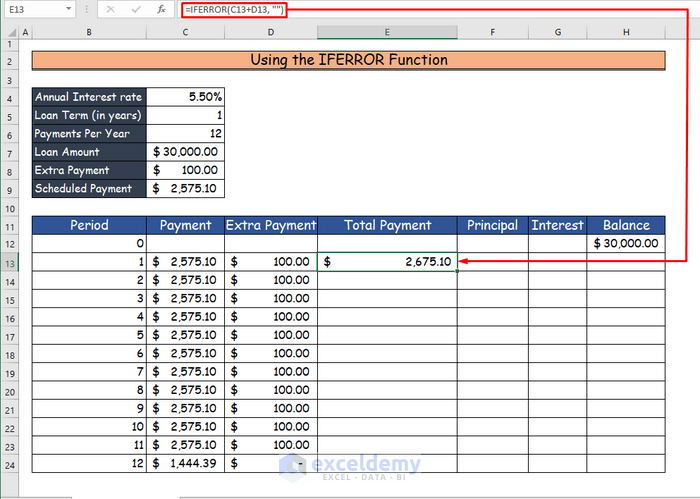
=IFERROR(C13+D13, "")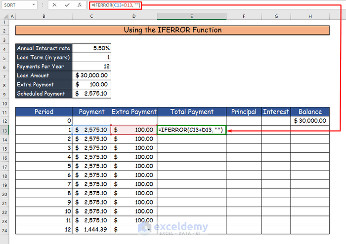
- Then, press Enter and you will get the total payment for the first month in cell E13, which is $2,675.10.
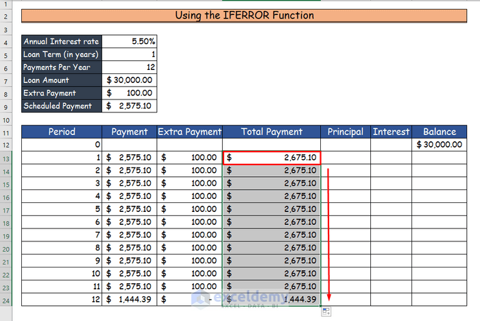
- Lastly, use AutoFill to drag the formula to the lower cells in the column.
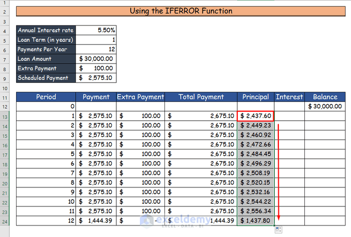
- Now, determine the principal in column F by using the IFERROR function.
=IFERROR(IF(C13>0, MIN(C13-G13, H12), 0), "")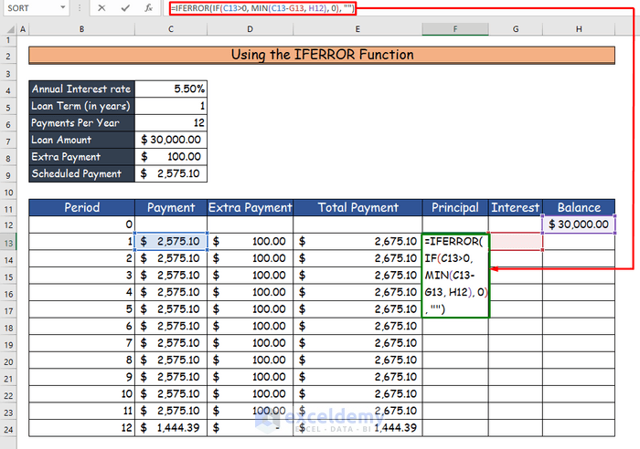
- Then, press Enter and get the principal for the first month in cell F13, which is $2,437.60.

- Lastly, drag the formula to the lower cells of the column.
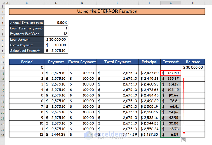
- In this step, calculate the interest.
- Apply the following formula based on the IFERROR function.
=IFERROR(IF(C13>0, $C$4/$C$6*H12, 0), "")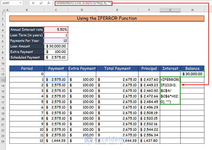
- Then, press Enter and get the value of the interest in cell G13, which is $137.50.

- Finally, use AutoFill to drag the formula to the lower cells in column G.
- In the final step, calculate the balance in column H by using the IFERROR function.
=IFERROR(IF(H12 >0, H12-F13-D13, 0), "")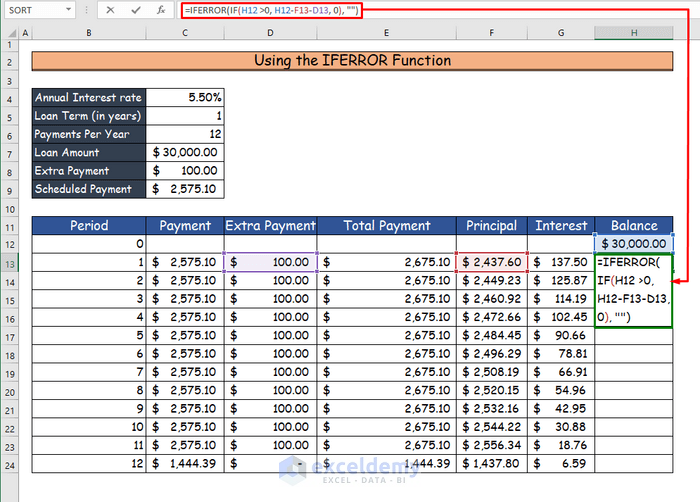
- Then, press Enter and get the value for the balance in cell H13, which is $ 27,462.40.
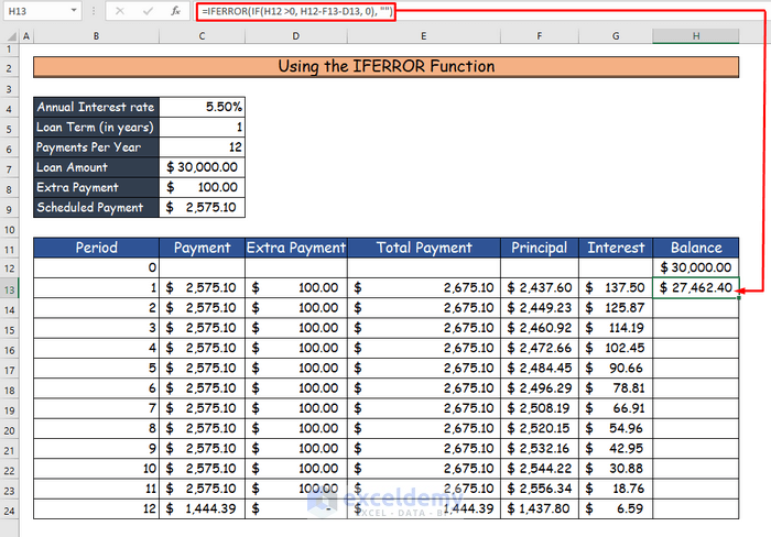
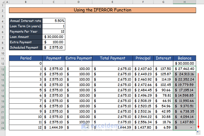
- Drag the formula to the lower cells in column H.
- You can see that, after the 12th installment, you will be able to repay the loan with extra payments.
2. Combining PMT, IPMT, and PPMT Functions to Create an Excel Loan Calculator with Extra Payments
If the loan amount, interest rate, and the number of periods are present, then you can calculate the required payments that will fully repay the loan by using the PMT function. PMT means payment in finance. We will use the PMT function to create an Excel loan calculator with extra payments. Along with the PMT function, we will also demonstrate the use of Excel’s interest payment function (the IPMT function) and principal payment function (the PPMT function) in this procedure.
Steps:
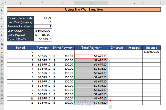
- Firstly, calculate the payment (PMT) in cell C9.
- To do this, apply the following formula using the PMT function.
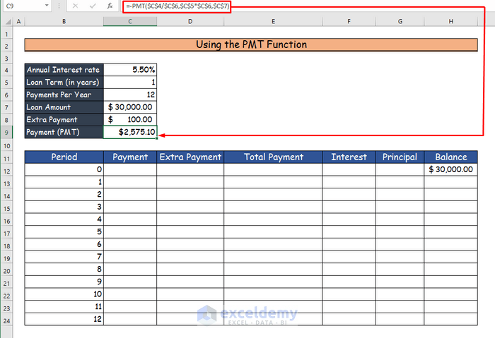
=-PMT($C$4/$C$6,$C$5*$C$6,$C$7)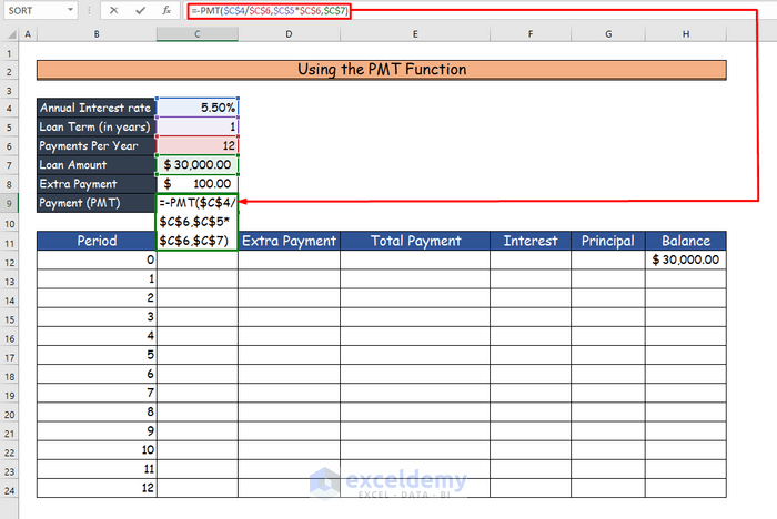
- Then, press Enter and you will get the scheduled payment in cell C9, which is $2,575.10.
- Now, accommodate the value of payment in cell C13, which is equal to the value of cell C9.
=$C$9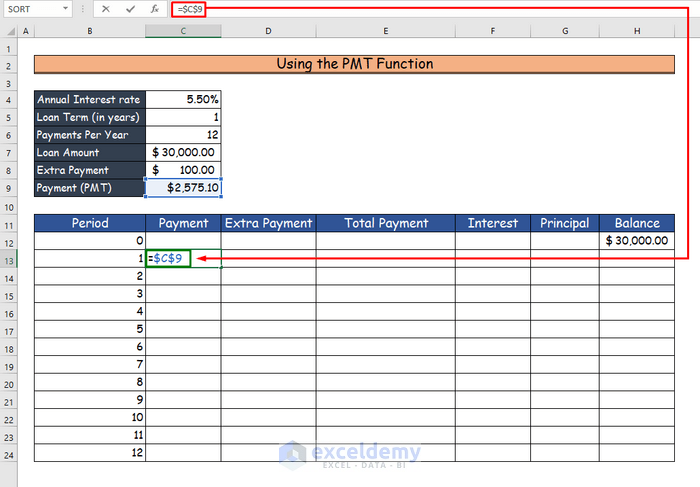
- After that, press Enter and you will get the payment for the first month in cell C13, which is $2575.10.
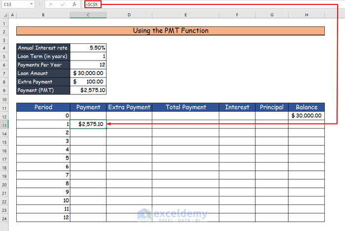
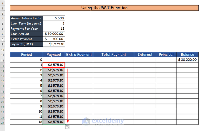
- Finally, drag the formula to the lower cell in column C using AutoFill tool.
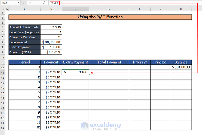
- Then, put the value of the extra payment in column D, which is equal to the value of cell C8.
=$C$8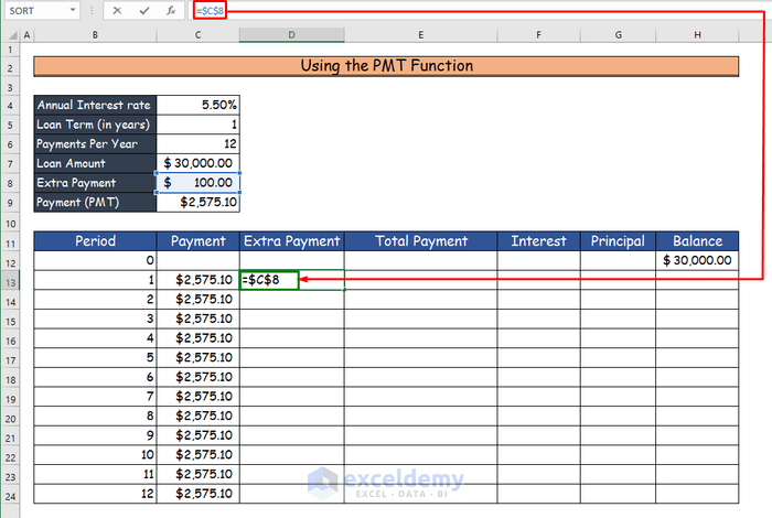
- Then, press Enter and you will get the extra payment for the first month in cell D13, which is $100.
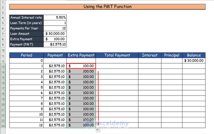
- Finally, to fill up the lower cells of that column, use AutoFill.
- Here, calculate the total payment in column E by applying the following formula.
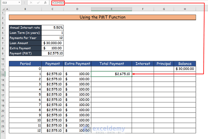
=C13+D13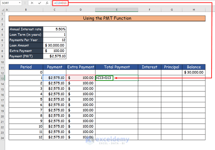
- Then, press Enter and you will get the total payment for the first month in cell E13, which is $2,675.10.
- Lastly, use the AutoFill feature to drag the formula to the lower cells in column E.
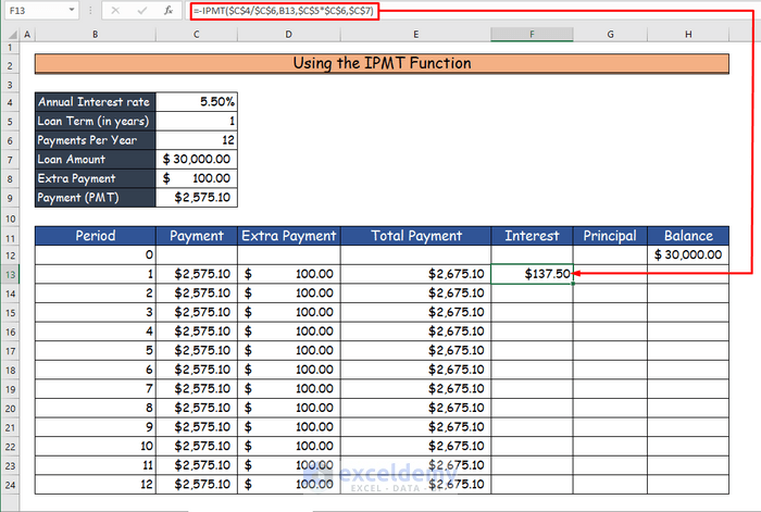
- Now, determine the interest in column F with the IPMT function formula below.
=-IPMT($C$4/$C$6,B13,$C$5*$C$6,$C$7)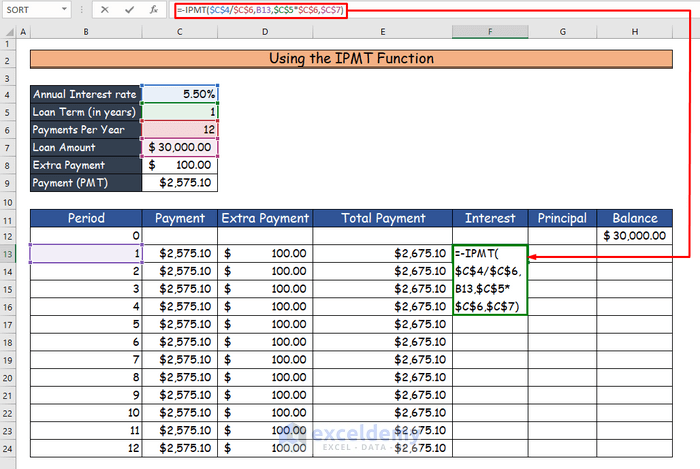
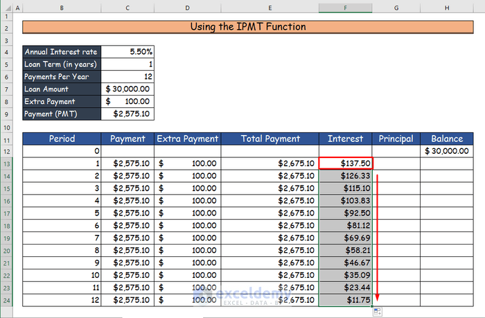
- Then, press Enter and get the interest for the first month in cell F13, which is $137.50.
- Lastly, use the Autofill to fill the lower cells with values in column F.
- In this step, calculate the principal in column G while inserting the PPMT function.
=-PPMT($C$4/$C$6,B13,$C$5*$C$6,$C$7)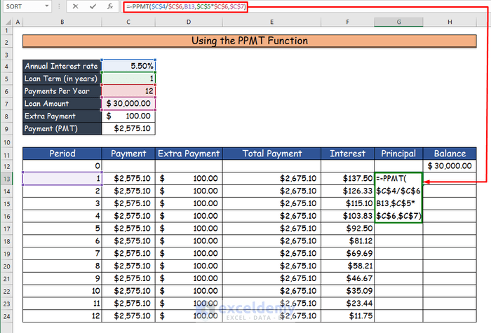
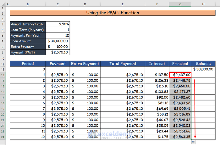
- Then, press Enter and get the value of the principal in cell G13, which is $2437.60.

- Finally, use the AutoFill and fill the lower cells with values.
- In the final step, calculate the balance in column H by using the following formula.
=H12-G13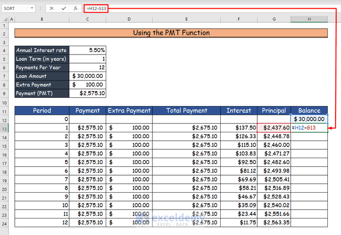
- Then, press Enter and get the value for the balance in cell H13, which is $ 27,562.40.

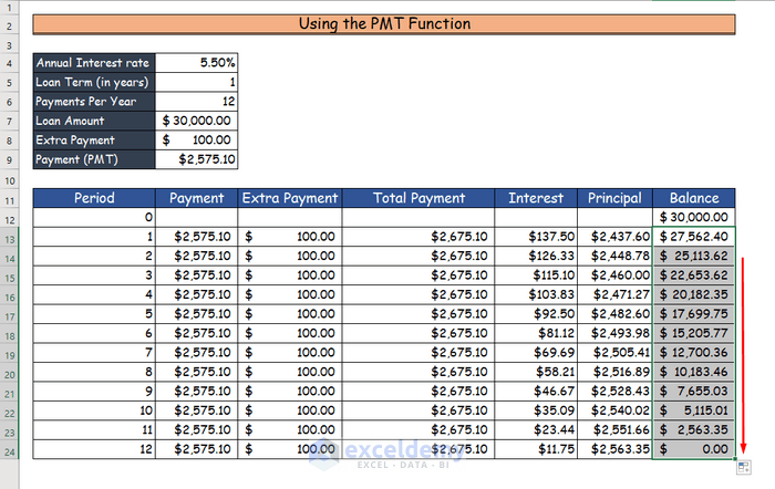
- Finally, use AutoFill to drag the formula to the lower cells in column H.
- You can see that, after the 12th installment, you will be able to repay the loan with extra payments.
- Use a minus (-) sign before the PPT, IPMT, and PPMT functions. In this way, the value from the formula will be positive and therefore easier to calculate.
- Use absolute cell reference where the input value is fixed or unchangeable for the lower cells. Otherwise, you will not get the desired result.
Download Practice Workbook
You can download the free Excel workbook from here and practice on your own.
Conclusion
That’s the end of this article. I hope you find this article helpful. After reading this article, you will be able to create an Excel loan calculator with extra payments by using any of these methods. Please share any further queries or recommendations with us in the comments section below.
Related Articles
- Create Home Loan Calculator in Excel Sheet with Prepayment Option
- Excel Simple Interest Loan Calculator with Payment Schedule
- Car Loan Calculator in Excel Sheet
<< Go Back to Loan Calculator | Finance Template | Excel Templates
Get FREE Advanced Excel Exercises with Solutions!
