How to Change Lowercase to Uppercase in Excel Without Formula

If you are facing problems in changing lowercase to uppercase or vice versa in Excel without formula, and you want to overcome the problems, then you are in a right place. In this tutorial, you will learn 5 effective methods to change cases without formula in Excel with proper illustrations.

How to Change Lowercase to Uppercase in Excel without Formula: 5 Methods

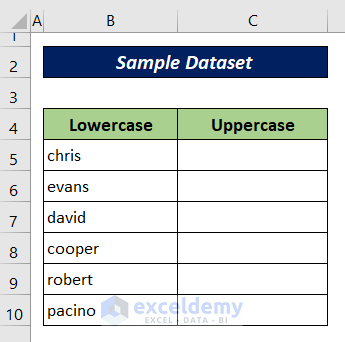
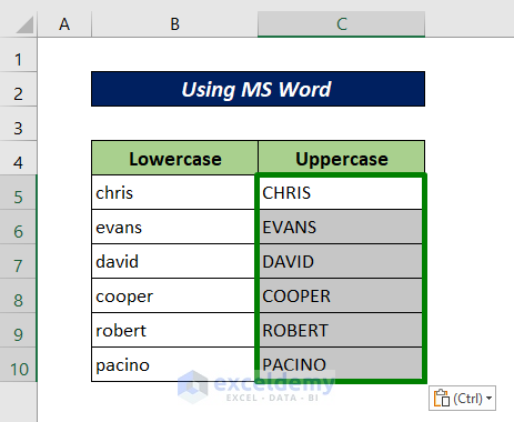
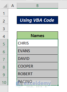
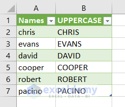
Here, we have a data set containing two columns. Our goal is to change lowercase texts on the left column to uppercase on the right blank column. 

1. Use the Flash Fill Feature

Flash Fill senses the pattern in your text and fills your data in this way. It identifies the cell value pattern and repeats the order for the rest of the cells. 

To change the lowercase letters to uppercase with the Flash Fill feature, follow the steps below.

Steps:

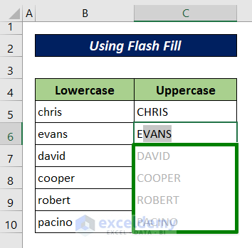
• First of all, type the first lowercase text “chris” (which is in Cell B5) in Cell C5 in uppercase format, i.e. “CHRIS“. Then press Enter.
• Press Alt+E to activate the Flash Fill.
• Now, start to type E (for EVANS).

You see, MS Excel suggests the rest. Not only that, but Flash Fill also suggests the rest of the names if they are to be typed in the same manner.

• Just accept the suggestion by pressing Enter.

Read More: How to Change Lowercase to Uppercase with Formula in Excel

2. Use Excel Caps Fonts

When you always want a text in uppercase and you don’t want to worry about how the text will be typed, you can use a font that has no lowercase style of the letters. The following fonts are always in the uppercase version of the letters. 

Steps:

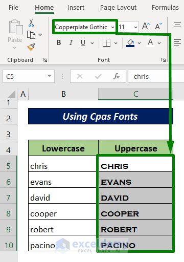
• Under the Home tab, select a font of the above list from the font dropdown list or type the font name on the box. Here, I have chosen Copperplate Gothic. 
• Now type anything; here, the names, not worrying about the case anymore (it will be written in uppercase automatically now).

Note:

The output is always in an uppercase style whether you type your text in lowercase, mixed-case, or uppercase.

Read More: Change Case for Entire Column in Excel

3. Change Lowercase to Uppercase in Excel with the Help of Microsoft Word

If you don’t feel comfortable using formulas in Excel, you can apply a system for converting text cases in MS word. Just follow the steps below.

Steps:

• Copy the range of cells i.e. B5:B10 that you want to change cases in Excel. 
• Open an MS Word document.
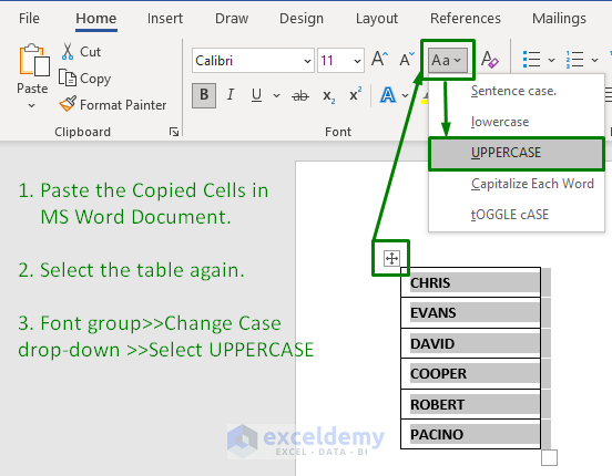
• Paste the copied cells in it.
• Select the texts that you want to change cases.
• Under the Home tab, click on the Change Case icon. Pick UPPERCASE options from the list.

• Now copy the text from the word table.
• Right-click on Cell C5.
• Select the paste option as in the following image.

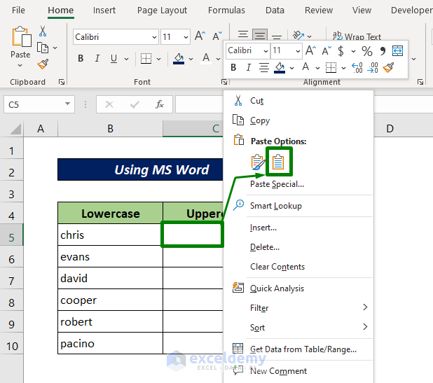
Here is the result.

4. Use an Excel VBA Code to Convert Letters to Uppercase

If you feel comfortable using the VBA codes in Excel, then copy the following code and paste it into the code module, and finally Run the code to get the result. 

Steps:

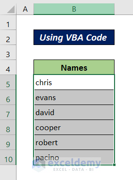
• Select the column in which you want to change the case.

• Press Alt+F11 and a VBA module will open.

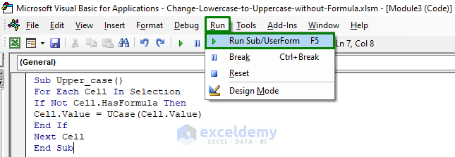
• Paste the following code in the module.

Sub Upper_case()
For Each Cell In Selection
If Not Cell.HasFormula Then
Cell.Value = UCase(Cell.Value)
End If
Next Cell
End Sub

• Then press Run Sub/UserForm, or just press F5.

Here is the result.

Notes: To apply Lowercase, insert the following code into the Module window.

Sub Lower_case()
For Each Cell In Selection
If Not Cell.HasFormula Then
Cell.Value = LCase(Cell.Value)
End If
Next Cell
End Sub

Again to apply Propercase, insert the following code into the Module window.

Sub Proper_case()
For Each Cell In Selection
If Not Cell.HasFormula Then
Cell.Value = _
Application _
.WorksheetFunction _
.Proper(Cell.Value)
End If
Next Cell
End Sub

Read More: Change Upper Case to Lower Case in Excel

5. Use the Power Query Tool to Change Lowercase to Uppercase

Power query is a significant tool for data transformation. By applying Power Query, we can convert the case into lowercase, uppercase, and propercase styles. Follow the steps below.

Steps:

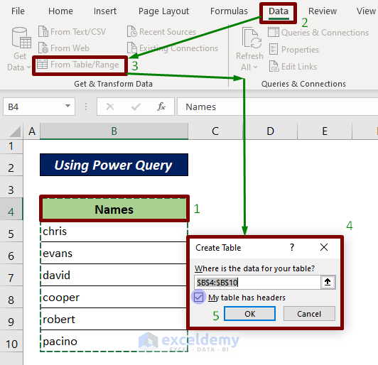
• Select any cell in the dataset.
• Go to the Data tab> From Table/Range.

A pop-up will appear.

• Mark My table has headers option.
• Check the data range as shown in the screenshot below.
• Press OK.

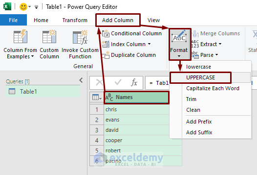
• A Power Query Editor window will pop up.
• Ensure the column is selected, then go to Add Column> Format> UPPERCASE. A new UPPERCASE column will be created beside the previous lowercase column.

• Now go to the File tab> Close & Load.

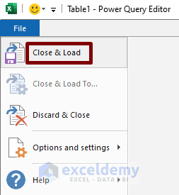
• The following table will be created in your Excel file in an additional worksheet.

Download Practice Book

Download the following Excel file for your practice.

Conclusion

In this tutorial, I have discussed 5 easy methods of how to change lowercase to uppercase in excel without formulas. I hope you found this tutorial helpful. Please, drop comments, suggestions, or queries if you have any in the comment section below. 

Related Articles

• How to Change Case in Excel Sheet
• How to Change Sentence Case in Excel
• Make First Letter of Sentence Capital in Excel
  
• Excel VBA to Capitalize First Letter of Each Word
• Capitalize First Letter of Each Word in Excel

<< Go Back to Change Case | Text Formatting | Learn Excel