10 Excel Tips Every Office Worker Should Know

Image by Editor
 

Microsoft Excel is one of the most useful and essential productivity tools in every workplace. Whether you’re tracking budgets, organizing data, or analyzing reports, knowing how to use Excel efficiently can save you hours of work.

In this article, we will list 10 Excel tips every office worker should know.

1. Master Keyboard Shortcuts

Learning keyboard shortcuts will dramatically increase your efficiency in Excel. You can perform tasks with simple clicks.

• Ctrl+C and Ctrl+V: Copy and paste.
• Ctrl+Z: Undo last action.
• Ctrl+S: Save.
• Ctrl+Arrow Keys: Navigate to the edge of data regions.
• Ctrl+Shift+Arrow Keys: Select data to the edge of the content.
• F2: Edit the selected cell.
• Alt+=: AutoSum (quickly add up a column or row).
• Ctrl+1: Open Format Cells dialog box.
• Alt + =: AutoSum.

2. Use Flash Fill

Flash Fill automatically fills data when it detects a pattern without using complex formulas. Simply start typing the pattern in the column next to your data, and Excel will suggest the remaining values.

Common use of Flash Fill:

• Splitting full names into first and last names.
• Extracting parts of text from a cell.
• Formatting phone numbers, SSNs, or other standardized data.

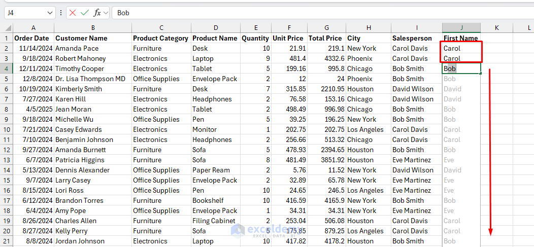
Let’s split the sales rep names from our sample data into first and last names:

• In column J (a blank column), type Carol (extracting just the first name from Carol Davis ).
• Start typing Carol in cell J3.
• Type Bob in cell J4.
• Excel will recognize the pattern and suggest filling the rest of the column with first names.
• Press Enter to accept.

Or

• Type the last name in K2.
• Press Ctrl + E or go to Data tab >> click Flash Fill.

3. Freeze Panes for Better Navigation

When working with large datasets, freezing panes keeps important row or column headers visible as you scroll.

• Select the cell below and to the right of where you want to freeze.
• Go to View tab >> from Freeze Panes >> select Freeze Panes.

Let’s freeze the top rows (Header row):

• Select the Header row.
• Go to View tab >> from Freeze Panes >> select Freeze Top Row.

This keeps your headers in view while navigating through large spreadsheets.

4. Convert Data to Tables

Tables in Excel provide numerous benefits; they convert the data into a structured format that helps to do further calculations and analysis.

Table offers:

• Automatic formatting with alternating row colors.
• Filter arrows in headers.
• Dynamic range expansion.

Let’s convert our sales data to a table:

• Select your data range.
• Go to the Insert tab >> select Table or press Ctrl+T.
• Check My table has headers.
• Click OK.

Use Table Features:

• Add a Total Row: Table Design → Check “Total Row”
  • The total row appears at the bottom with the sum of sales.
• Use structured references in formulas: Instead of writing =SUM(H2:H11), you can write =SUM(Table1[Total]), which automatically updates if rows are added.
• Quick Analysis: Click on your table and use the Quick Analysis button that appears in the bottom right to quickly create charts, totals, or formatting based on your data.

5. Master VLOOKUP (or XLOOKUP)

VLOOKUP is essential for finding data in large tables. It searches for a value from one column and returns a related value from another.

Syntax:

=VLOOKUP(lookup_value, table_array, column_index_num, [range_lookup])

Let’s find out the product price:

Formula:

=VLOOKUP(A2,Sales_Data!$F$2:$H$71,3, FALSE)

This formula looks for the product name entered in cell A2 within the first column (column F) of the range F2:H71 on the Sales_Data sheet. Once it finds a match, it returns the value from the 3rd column of that range, which is column H that contains the unit price.

For newer Excel versions, XLOOKUP is even more powerful:

Syntax:

=XLOOKUP(lookup_value, lookup_array, return_array, [if_not_found], [match_mode], [search_mode])

Formula:

=XLOOKUP(A2,Sales_Data!$F$2:$F$71,Sales_Data!$H$2:$H$71,"Not Found",0)

This formula searches for the product name in cell A2 within the lookup array F2:F71 and returns the corresponding unit price from the return array H2:H71. If the product is not found, it displays “Not Found”.

XLOOKUP is better because it’s easier to read, doesn’t require column numbers, can search both left and right, handles errors directly, and is more flexible if the data structure changes.

These functions help you find and pull data from other parts of your workbook without manual searching.

6. PivotTables for Data Analysis

PivotTables quickly summarize and analyze large datasets.

PivotTables are perfect for:

• Summarizing data by categories.
• Creating cross-tabulations.
• Identifying trends and patterns.
• Performing calculations on grouped data.

Let’s create a PivotTable to analyze sales:

• Click anywhere in your data.
• Go to the Insert tab >> select PivotTable.

• In the PivotTable Field List:
  • Drag City to the Rows field.
  • Drag the Product Name to the Columns field.
  • Drag Total Price to the Values field.

This instantly shows:

• Houston city has the highest total sales ($19801.48).
• Some notable large individual sales include:
  • Houston’s Laptop sales $4,954.73.
  • New York’s Bookshelf sales $4,711.06.
  • Phoenix’s Filing Cabinet sales $4,332.6.

7. Conditional Formatting

Conditional formatting helps visualize data and identify patterns. You can highlight important data like deadlines, targets, or duplicates.

• You can use Data Bars, Color Scales, or Icon Sets in your data.
• You can also create custom rules to highlight specific values, date ranges, or text.

Let’s apply conditional formatting to our sales data to highlight high-value orders:

• Select the Total Price column.
• Go to Home tab >> select Conditional Formatting >> select Color Scales >> select Green-Yellow-Red Color Scale.

The same column now shows a visual gradient:

• The highest values appear green.
• Medium values appear yellow.
• Lower values appear red.

 Custom Rule: To highlight all sales over $1000:

• Select the data range.
• Go to the Home tab >> select Conditional Formatting >> select New Rule.
• Select Format only cells that contain.
• Set Cell Value >> greater than or equal to >> 1000
• Choose a bold blue fill color.
• Click OK.

Now, all sales equal to or greater than $1000 will be highlighted in blue, making them instantly visible.

8. Use Filters and Slicers

Filters help you focus on specific data. To search for specific values from a large dataset filter option is super useful.

If you are using Table or PivotTable:

• Click the filter button in your header row or table.
• Use the dropdown menus to select criteria.

If you want to filter the normal dataset:

• Select the data range.
• Go to the Data tab >> select Filter or press CTRL+SHIFT+L.

Let’s filter sales based on City:

• Click the filter button on the City column.
• Uncheck Select All >> check only Houston.
• Click OK.

The filtered result shows only Houston city sales.

Slicers:

For more interactive filtering, you can use Slicers with a Table or PivotTable:

• Select your table or PivotTable.
• Go to the Insert tab >> select Slicer.
• Check Salesperson and City.
• Click OK.

• Select salesperson Bob Smith.
• Select city Chicago.

This provides a dashboard-like experience for exploring your data without having to open filter dropdowns repeatedly.

9. Text to Columns

When you need to split data in a single column into multiple columns, you can use the Text to Columns feature. It is useful when we import data from various sources, especially CSV files.

• Select the column with data to split.
• Go to the Data tab >> select Text to Columns.
• Choose Delimited (for splitting by commas, tabs, etc.) or Fixed Width.
• Follow the wizard to specify how to split your data.

This is perfect for separating names, addresses, or imported data.

• Select column A containing the customer data.
• Go to Data tab >> select Text to Columns.
• Choose Delimited >> click Next.

• Check Comma as the delimiter >> click Next.

• Choose formatting for each column (General is fine) >> click Finish.

Output:

This method works well when you need to split fixed formats like:

• Full addresses into street, city, state, zip.
• Product codes into category, subcategory, and ID.
• CSV data imported as a single column.

10. Data Validation

Data validation ensures data integrity and can create dropdown lists for consistent data entry.

Prevent errors by limiting what can be entered in cells:

• Select the cells you want to restrict.
• Go to Data tab >> select Data Validation.
• Set up rules (e.g., whole numbers between 1-100, dates, or a list of specific options).
• Add input messages and error alerts.

Let’s create a dropdown list for City when adding new entries:

• List the city name in the empty column end of the dataset or another sheet.
• Select cell D2 (where you’d add a new entry).
• Go to Data tab >> select Data Validation.
• Under Allow, select List.
  • Select the city range: $L$2:$L$6
• Click OK.

Now, cell D2 has a drop-down that only allows listed cities.

• Users can’t enter invalid regions.
• The dropdown ensures consistency in data entry.

This technique works great for:

• Ensuring consistent category names.
• Limiting entries to acceptable ranges.
• Creating interactive forms in Excel.

Bonus Tip: Learn Basic Functions

These functions will make your Excel life easier:

• IF: Apply conditional logic to return values based on whether a condition is true or false.
• SUMIF/COUNTIF: Sum or count cells meeting specific criteria.
• INDEX/MATCH: More flexible alternative to VLOOKUP.
• CONCATENATE or &: Join text from different cells.
• DATE: Work with the date format.

Conclusion

These Excel tips are essential for office workers. Mastering these Excel tips will significantly improve productivity and make you more valuable in any office environment. Start practicing them one by one, and soon they’ll become second nature in your daily workflow.