How to Zoom in Excel Graph (With Easy Steps)

Written by Sabrina Ayon

Last updated: Dec 18, 2023

While working with Microsoft Excel, we insert graphs to make it possible to visualize data collections. We zoom an Excel graph to see it up close. The chart’s scale is enhanced, which enhances the readability of its values. In this article, we will demonstrate instructions to zoom in Excel graph gradually.

How to Zoom in Excel Graph: Step-by-Step Procedure

We may use graphs in Excel to visually convey information. People can absorb and recall information more easily with the aid of graphs. Many individuals comprehend images more rapidly than long passages of text. We may know how to add Excel graphs but many of us don’t have any idea how to zoom on those graphs. Let’s follow the instructions to do this.

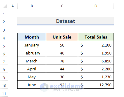
Step 1: Create Dataset

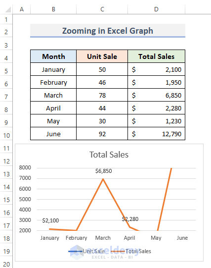
First, we need to create a dataset. As we know, the datasets are the continuous cell range holding data for analysis.

Firstly, we put some months in column B.
Secondly, insert the total unit sales of each month in column C.
And, finally, the total amount of sales for each particular month in column D.

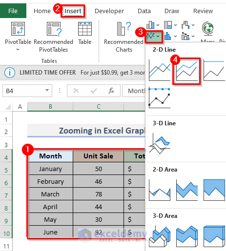
Step 2: Insert Graph

A graph can provide a sharper view of a set of data values. And, to zoom in on Excel graphs, we must insert the graph into our spreadsheet.

To begin with, we select the whole data that we have just created.
Then, go to the Insert tab from the ribbon.
Further, click on the Insert Line or Area Chart drop-down menu under the Charts group.
Consequently, choose the Stacked Line from the option, the second option of the 2-D Line list.

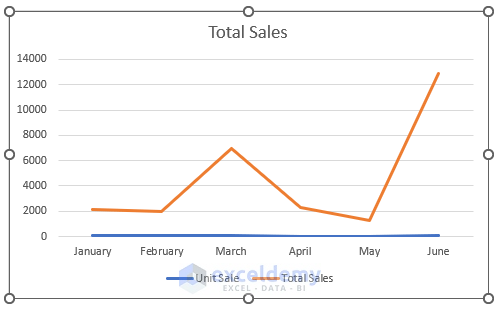
Thus, you can see the Total Sales graph in your spreadsheet.

Step 3: Display Format Axis

Format Axis add to explain what is presented on the axis, and is distinct from axis labels. Graphs may not always display axis titles. Format Axis works as a scale or comparison line for data plotted on a graph.

Click on the graph axis and right-click.
This will appear a context menu, from there click on Format Axis.

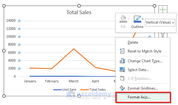
Thus the Format Axis dialog will show up on the right side of the spreadsheet.

Step 4: Set Axis Options

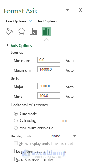
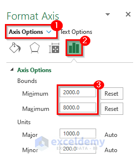
Now the main and the final step for zooming in on Excel graphs. In this step, we will set or edit the bounds of graph positions to zoom in on the graph.

In the first place, click on the Axis Options drop-down menu.
Then, under the menu click on the Axis Options which is the tiny bar icon.
Next from the Bounds category, set the Minimum and Maximum. This totally depends on how much you want to zoom in or zoom out on that graph.
By default, it was set automatically while plotting any graph. In our case, by default, the minimum bounds were 0.0 and the maximum bounds were 14000.0.
Now, we set the minimum bound 2000.0 and maximum bound 8000.0 to zoom in on the graph and have a close look at the graph.

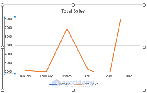
After doing this, we will see the graph is now zoomed in.

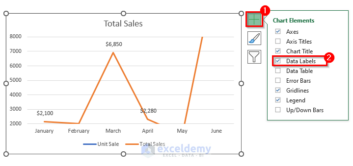
To have clearer visualization, we will click on the Chart Elements and checkmark the Data Labels to show the data on the graph.

Final Output

This is the final output after zooming in Excel graph.

Things to Keep in Mind

Consistently structure your X and Y axes to the lowest quality of the data for simplicity of use.
The chart will be simple to understand if the data labels, axis title, and data points are formatted correctly.

Download Practice Workbook

You can download the workbook and practice with them.

Zoom in Graph.xlsx

Conclusion

The above procedures will assist you to Zoom in Excel Graph. I hope this will help you! Please let us know in the comment section if you have any questions, suggestions, or feedback.

<<Go Back to How to Zoom in Excel | Excel Worksheets | Learn Excel

Get FREE Advanced Excel Exercises with Solutions!

Sub Zoom_Chart() Dim i As Integer Dim strButtonName As String Dim strChartName As String Dim strZoomState As String Dim dZoomInWidth As Double Dim dZoomInHeight As Double Dim dOutWidth As Double Dim dOutHeight As Double Dim rngZoom As Range Dim rngChart As Range Dim strZoomInText As String Dim strZoomOutText As String strZoomInText = "+" strZoomOutText = "-" dZoomInWidth = 3 dZoomInHeight = 2 dOutWidth = 1 / dZoomInWidth dOutHeight = 1 / dZoomInHeight strButtonName = Application.Caller Set rngZoom = Range(ActiveSheet.Shapes(strButtonName).TopLeftCell.Address) With ActiveSheet For i = 1 To .Shapes.Count strChartName = .Shapes(i).Name Set rngChart = Range(.Shapes(i).TopLeftCell.Address) If Not Intersect(rngZoom, rngChart) Is Nothing Then strZoomState = .Shapes(strButtonName).TextFrame.Characters.Text With ActiveSheet.Shapes(strChartName) If strZoomState = strZoomInText Then .ZOrder msoBringToFront .ScaleWidth dZoomInWidth, msoFalse, msoScaleFromTopLeft .ScaleHeight dZoomInHeight, msoFalse, msoScaleFromTopLeft ActiveSheet.Shapes(strButtonName).TextFrame.Characters.Text = strZoomOutText ActiveSheet.Shapes(strButtonName).ZOrder msoBringToFront Else .ScaleWidth dOutWidth, msoFalse, msoScaleFromTopLeft .ScaleHeight dOutHeight, msoFalse, msoScaleFromTopLeft ActiveSheet.Shapes(strButtonName).TextFrame.Characters.Text = strZoomInText End If End With GoTo EndLoop End If Next i End With EndLoop: End Sub

2 Comments

Joe Sep 28, 2023 at 3:42 AM

In excel 2016, my chart has multiple series with a common horizontal scale (think of a set of serial binary data signals over a time range). There are no “Bounds” minimum and maximum data entry fields. any thoughts?
- Reply
  Yousuf Khan Oct 3, 2023 at 10:06 AM
  Hello JOE,
  
  Thank you for sharing your experience with us. Since you have no Bounds command in your Excel 2016 version, let’s find an alternative way. Today, I am going to show you how to zoom your charts using VBA applicable in any Excel version. Let’s dive into it.
  
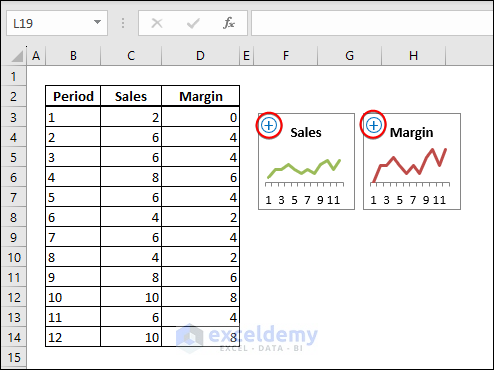
  1. First, create (+) and (-) buttons in your workbook >> name them Zoom_Button in the NameBox. Or, you can copy them from the attached workbook and paste them into your chart.
  
  2. Enter the below VBA code to your module >> Assign the Zoom_Chart macro in the buttons:
  (If you do not understand this step, see this article)
  How to Write VBA Code in Excel
  The VBA code:
```
Sub Zoom_Chart()

Dim i As Integer
Dim strButtonName As String
Dim strChartName As String
Dim strZoomState As String
Dim dZoomInWidth As Double
Dim dZoomInHeight As Double
Dim dOutWidth As Double
Dim dOutHeight As Double
Dim rngZoom As Range
Dim rngChart As Range
Dim strZoomInText As String
Dim strZoomOutText As String

        strZoomInText = "+"
        strZoomOutText = "-"
                                              
        dZoomInWidth = 3
        dZoomInHeight = 2
        dOutWidth = 1 / dZoomInWidth
        dOutHeight = 1 / dZoomInHeight
    
    strButtonName = Application.Caller
    
  
    Set rngZoom = Range(ActiveSheet.Shapes(strButtonName).TopLeftCell.Address)
    
    With ActiveSheet
        
        For i = 1 To .Shapes.Count
            strChartName = .Shapes(i).Name
            Set rngChart = Range(.Shapes(i).TopLeftCell.Address)
            
            If Not Intersect(rngZoom, rngChart) Is Nothing Then
                strZoomState = .Shapes(strButtonName).TextFrame.Characters.Text
                With ActiveSheet.Shapes(strChartName)
                    
                    
                    If strZoomState = strZoomInText Then
                        .ZOrder msoBringToFront
                        .ScaleWidth dZoomInWidth, msoFalse, msoScaleFromTopLeft
                        .ScaleHeight dZoomInHeight, msoFalse, msoScaleFromTopLeft
                        ActiveSheet.Shapes(strButtonName).TextFrame.Characters.Text = strZoomOutText
                        ActiveSheet.Shapes(strButtonName).ZOrder msoBringToFront
                   
                    Else
                        .ScaleWidth dOutWidth, msoFalse, msoScaleFromTopLeft
                        .ScaleHeight dOutHeight, msoFalse, msoScaleFromTopLeft
                        ActiveSheet.Shapes(strButtonName).TextFrame.Characters.Text = strZoomInText
                    End If
                End With
                GoTo EndLoop
            End If
        Next i
    End With

EndLoop:

End Sub
```
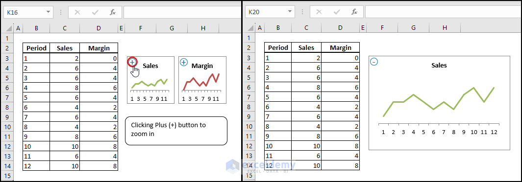
  3. Click the Plus (+) button to zoom in on your chart.
  
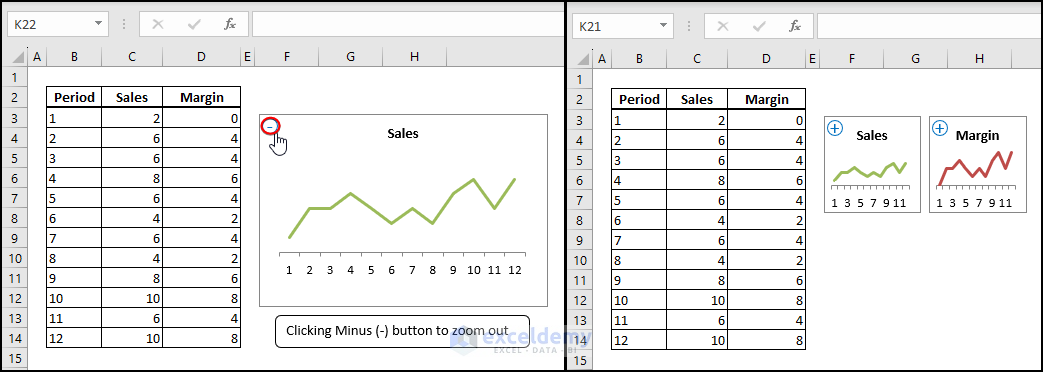
  4. Click the Minus (-) button to zoom out on your chart.
  
  You can set the zoom height and width in the given code in these lines:
```
dZoomInWidth = 3
dZoomInHeight = 2
```
  Note: Here, 3 means 300% zoom and 2 means 200% zoom.
  Download the workbook file here to practice.
  Zoom Excel Chart.xlsm
  Best Regards,
  Yousuf Khan Shovon