Task 1 – Data Cleaning and Formatting
1.1 Removing Blank Rows
Sometimes your dataset may have blank rows that you need to remove. However, removing them one by one can be tedious. We can write a few lines of VBA code to do the heavy lifting for us.
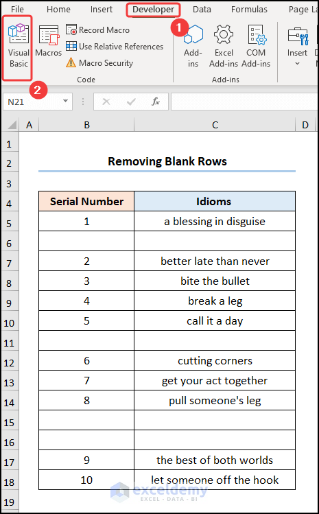
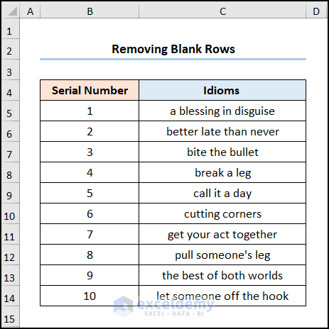
We have a sample dataset below of the List of Idioms in the B4:C14 cells.

Steps:
- Navigate to the Developer tab >> click on Visual Basic.
This opens the Visual Basic Editor in a new window.
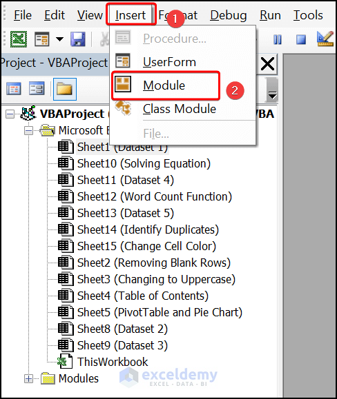
- Go to the Insert tab >> select Module.

Enter the following code into the window.
Sub Choose_Empty_Rows()
Dim row As Range
Dim choose As Range
Dim region As Range

  If TypeName(Selection) <> "Range" Then
    MsgBox "Choose a Range of Cells .", vbOKOnly, "Choose Empty Rows Macro"
    Exit Sub
  End If

  If Selection.Cells.Count = 1 Then
    Set region = ActiveSheet.UsedRange
  Else
    Set region = Selection
  End If

  For Each row In region.Rows
    If WorksheetFunction.CountA(row) = 0 Then
      If choose Is Nothing Then
        Set choose = row
      Else
        Set choose = Union(choose, row)
      End If
    End If
  Next row

  If choose Is Nothing Then
    MsgBox "Could not find any Blank Rows", vbOKOnly, "Choose Empty Rows Macro"
    Exit Sub
  Else
    choose.Select
  End If

End Sub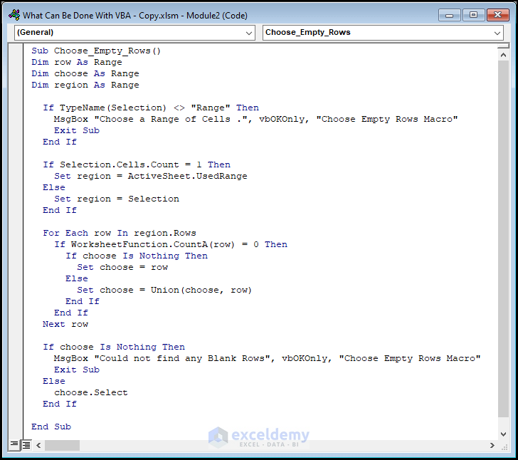
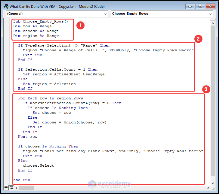
⚡ Code Breakdown:
- The sub-routine is given a name, here it is Choose_Empty_Rows().
- Define the variables row, choose, and region as Range.
- Use the If statement to check if a range has been selected.
- Use a second If statement to check whether multiple cells are present in the selected range.
- Combine the For Loop and If statements to loop through all the cells in the selected range and count the number of blank rows.
- Select the blank rows using the Select method. If there are no blank cells, it returns the message “Could not find any Blank Rows”.
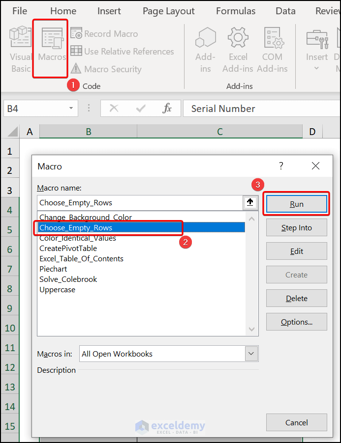
- Close the VBA window >> select the B4:C18 cells >> click Macros.
This opens the Macros dialog box.
- Select the Choose_Empty_Rows macro >> hit Run.
- All the blank rows are now selected >> press the CTRL + – (Minus) key >> select the Shift cells up option to delete the unwanted rows.
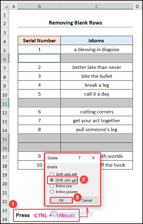
All selected blank rows will be deleted.
Read More: 20 Practical Coding Tips to Master Excel VBA
1.2 Changing Text to Uppercase
Steps:
- Go to the Developer tab >> click Visual Basic.
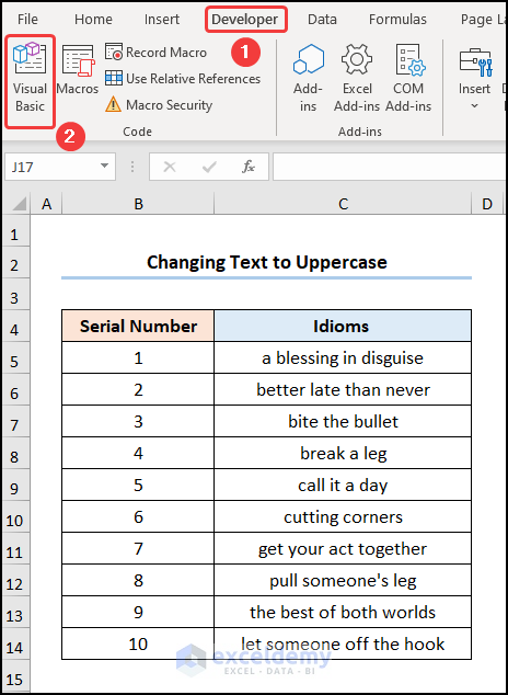
This opens the Visual Basic Editor in a new window.
- Navigate to the Insert tab >> choose Module.
Enter the following code into the window.
Sub Uppercase()

Dim i As Range
Set i = Selection
For Each cell In i
    cell.Value = UCase(Left(cell.Value, 1)) & Right(cell.Value, Len(cell.Value) - 1)
Next cell
End Sub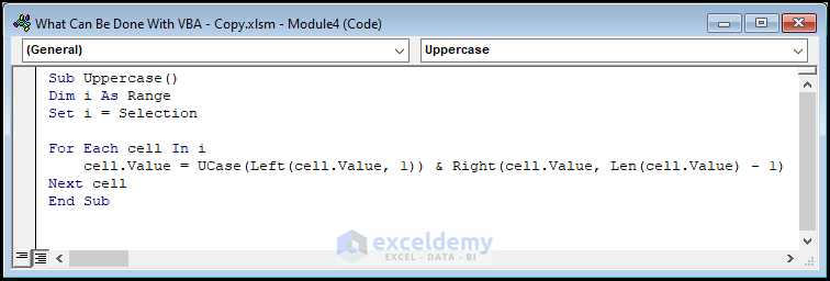
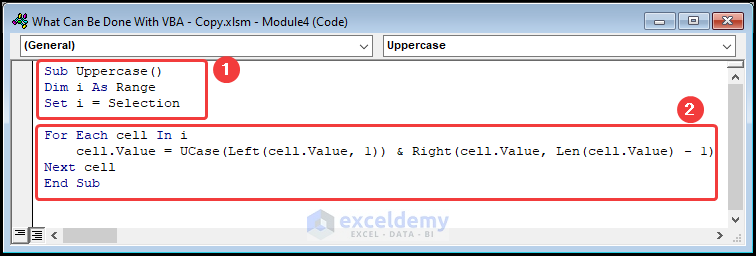
⚡ Code Breakdown:
- The sub-routine is given a name, and the variables are defined.
- Assign the Selection property to the variable i. This allows us to choose a range of cells where we can perform operations.
- We use a For loop to run the UCase function which capitalizes the first letter extracted by the LEFT function and joins it with the text returned by the RIGHT function.
- Close the VBA window >> select column C >> click on Macros.
- Choose the Uppercase Macro >> press the Run button.
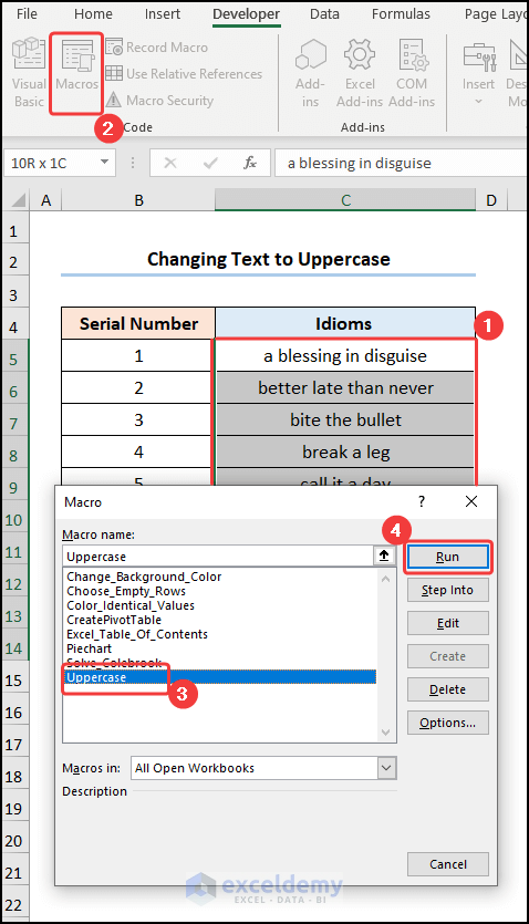
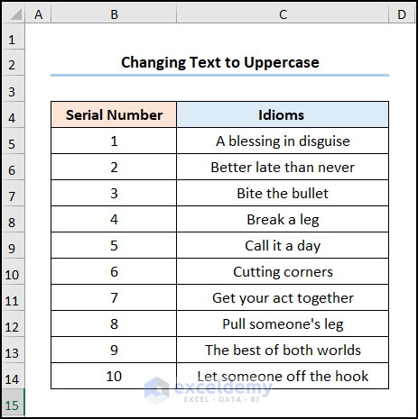
The first letters of the text in the cells will change to uppercase.
Task 2 – Worksheet-Related Tasks
2.1 Creating Table of Contents
Steps:
- Open the Visual Basic editor, insert a new Module and enter the following code.
Sub Excel_Table_Of_Contents()

    Dim alerts As Boolean
    Dim y  As Long
    Dim Wrksht_Index As Worksheet
    Dim Wrksht As Variant

    alerts = Application.DisplayAlerts
    Application.DisplayAlerts = False
    On Error Resume Next
    Sheets("Table of contents").Delete
    On Error GoTo 0
    Set Wrksht_Index = Sheets.Add(Sheets(1))
    Wrksht_Index.Name = "TOC"
    y = 1
    Cells(1, 1).Value = "TOC"
    For Each Wrksht In ThisWorkbook.Sheets
        If Wrksht.Name <> "Table of contents" Then
            y = y + 1
            Wrksht_Index.Hyperlinks.Add Cells(y, 1), "", "'" & Wrksht.Name & "'!A1", , Wrksht.Name
        End If
    Next
    Application.DisplayAlerts = alerts
End Sub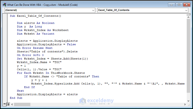
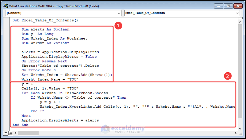
⚡ Code Breakdown:
- The sub-routine is given a name, here it is Excel_Table_Of_Contents().
- Define the variables alerts, y, and Wrksht.
- Assign Long, Boolean, and Variant data types respectively.
- Define Wrksht_Index as the variable for storing the Worksheet object.
- Remove any previous Table of Contents sheet using the Delete method.
- Insert a new sheet with the Add method in the first position and name it “Table of contents” using the Name statement.
- We declare a counter (y = 1) and use the For Loop and the If statement to obtain the names of the worksheets.
- Use the HYPERLINK function to generate clickable links embedded in the worksheet names.
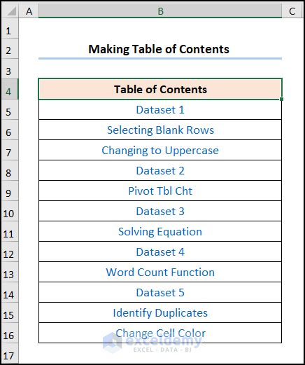
- Click the Run button or press the F5 key to run the macro.
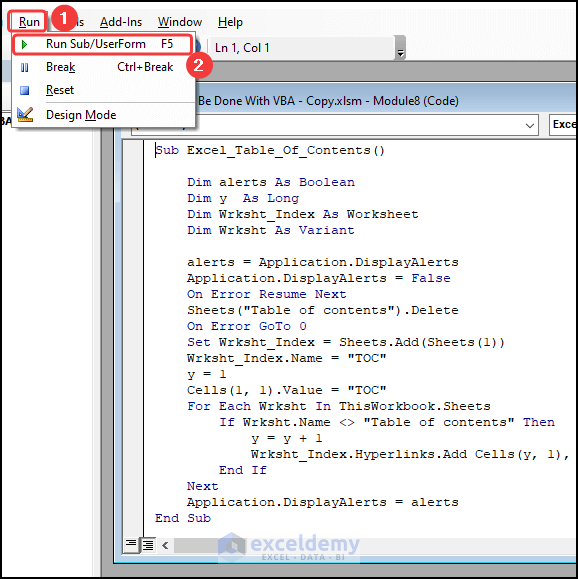
A table of contents will be created.
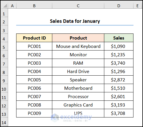
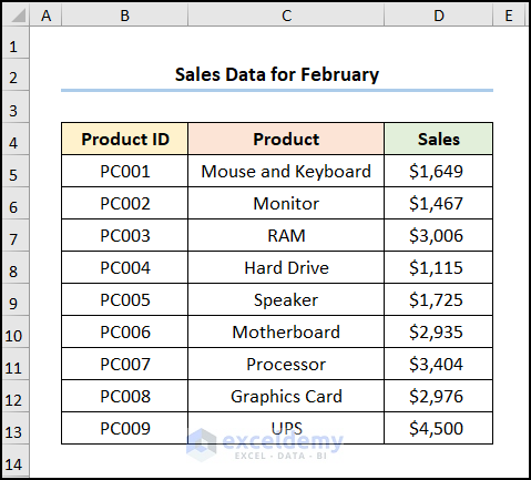
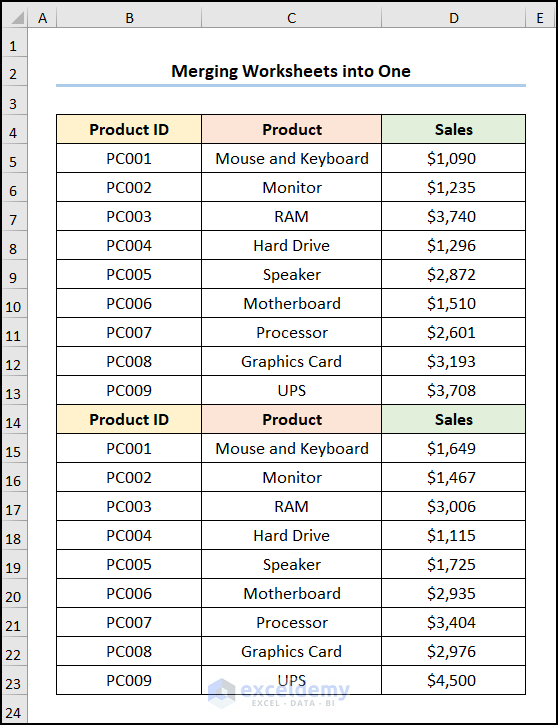
2.2 Merging Multiple Worksheets into One
We have two sample datasets. One for the month of January.
Another for February, as shown below.
Steps:
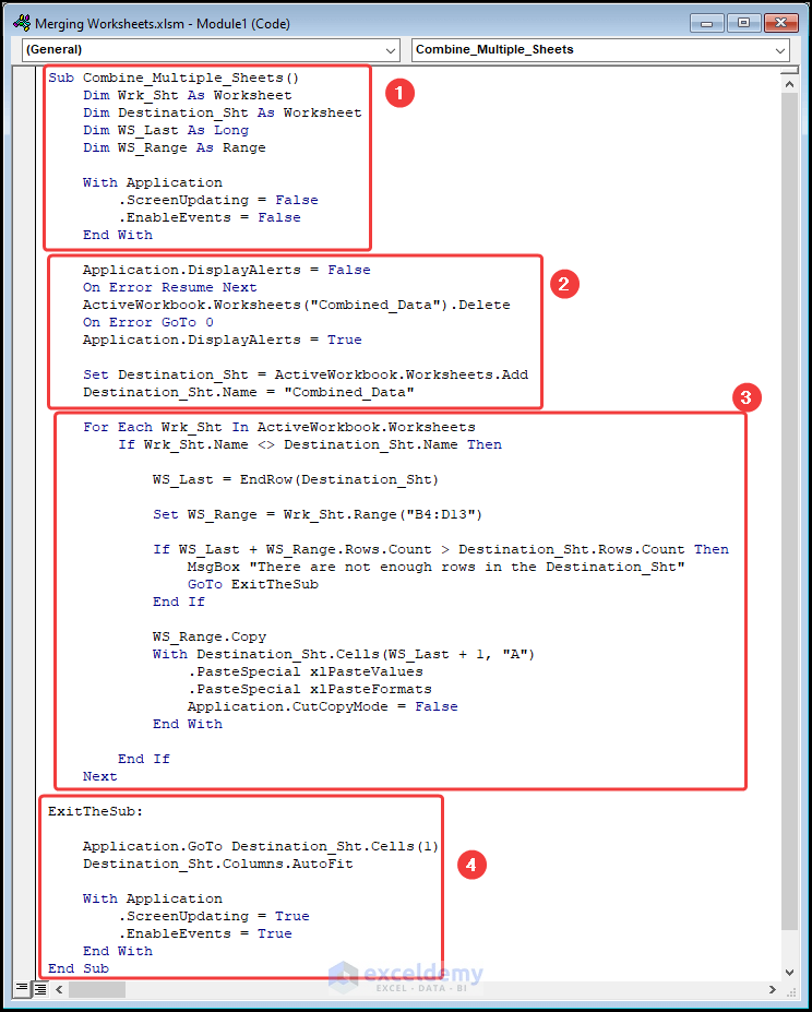
- Open the Visual Basic editor, insert a new Module and enter the code.
Sub Combine_Multiple_Sheets()
    Dim Wrk_Sht As Worksheet
    Dim Destination_Sht As Worksheet
    Dim WS_Last As Long
    Dim WS_Range As Range

    With Application
        .ScreenUpdating = False
        .EnableEvents = False
    End With

    Application.DisplayAlerts = False
    On Error Resume Next
    ActiveWorkbook.Worksheets("Combined_Data").Delete
    On Error GoTo 0
    Application.DisplayAlerts = True

    Set Destination_Sht = ActiveWorkbook.Worksheets.Add
    Destination_Sht.Name = "Combined_Data"

    For Each Wrk_Sht In ActiveWorkbook.Worksheets
        If Wrk_Sht.Name <> Destination_Sht.Name Then

            WS_Last = EndRow(Destination_Sht)

            Set WS_Range = Wrk_Sht.Range("B4:D13")

            If WS_Last + WS_Range.Rows.Count > Destination_Sht.Rows.Count Then
                MsgBox "There are not enough rows in the Destination_Sht"
                GoTo ExitTheSub
            End If

            WS_Range.Copy
            With Destination_Sht.Cells(WS_Last + 1, "A")
                .PasteSpecial xlPasteValues
                .PasteSpecial xlPasteFormats
                Application.CutCopyMode = False
            End With

        End If
    Next

ExitTheSub:

    Application.GoTo Destination_Sht.Cells(1)
    Destination_Sht.Columns.AutoFit

    With Application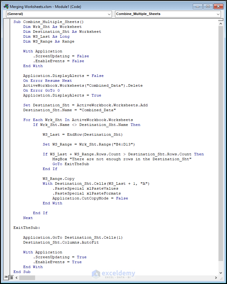
⚡ Code Breakdown:
- Name the sub-routine, here it is Combine_Multiple_Sheets().
- Define the variables and assign Long and Range data types respectively.
- Delete the Combined_Data worksheet if it already exists.
- Add a new worksheet with the name Combined_Data.
- Use the For Loop and the If statement to loop through every spreadsheet and copy-paste the data into the Combined_Data worksheet.
- Use the AutoFit method to fit the data in the Combined_Data worksheet.
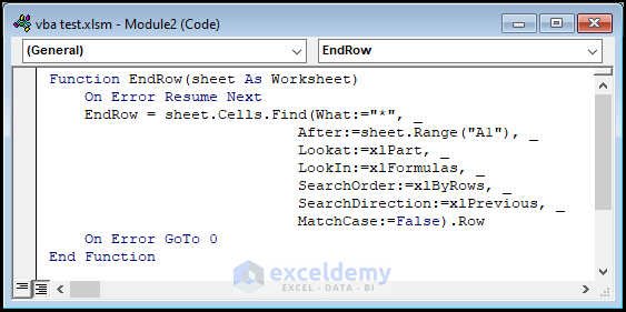
- Insert a second Module >> Enter the following VBA code into the window.
Function EndRow(sheet As Worksheet)
    On Error Resume Next
    EndRow = sheet.Cells.Find(What:="*", _
                            After:=sheet.Range("A1"), _
                            Lookat:=xlPart, _
                            LookIn:=xlFormulas, _
                            SearchOrder:=xlByRows, _
                            SearchDirection:=xlPrevious, _
                            MatchCase:=False).Row
    On Error GoTo 0
End Function
The EndRow function locates the last row in the Combined_Data worksheet.
- Choose the Combine_Multiple_Sheets macro and click on Run.
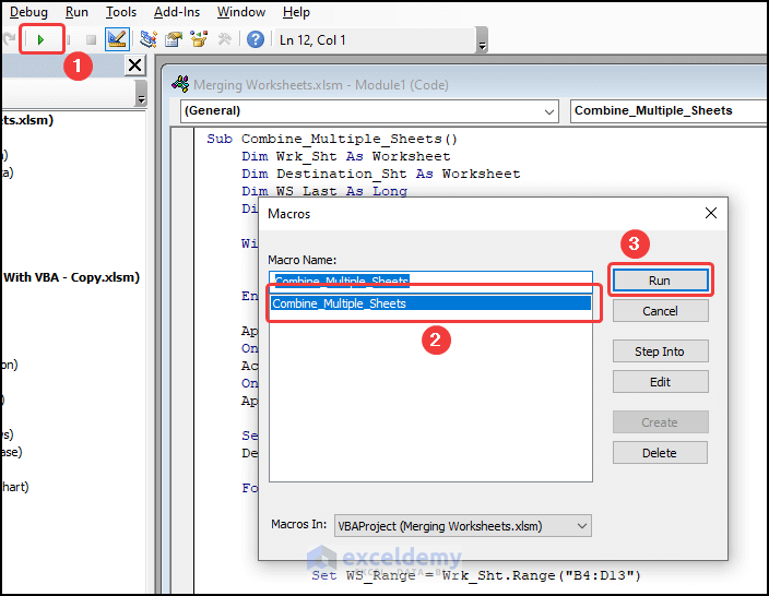
The two worksheets will be combined into one.
Task 3 – Automating PivotTables and PivotCharts
Steps:
- Follow Steps 1-2 from the previous tasks.
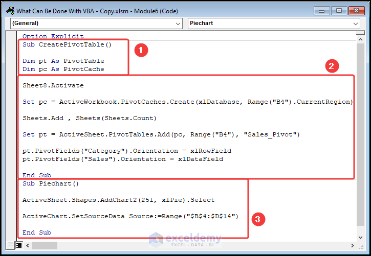
Option Explicit
Sub CreatePivotTable()

Dim pt As PivotTable
Dim pc As PivotCache

Sheet8.Activate

Set pc = ActiveWorkbook.PivotCaches.Create(xlDatabase, Range("B4").CurrentRegion)

Sheets.Add , Sheets(Sheets.Count)

Set pt = ActiveSheet.PivotTables.Add(pc, Range("B4"), "Sales_Pivot")

pt.PivotFields("Category").Orientation = xlRowField
pt.PivotFields("Sales").Orientation = xlDataField

End Sub
Sub Piechart()

ActiveSheet.Shapes.AddChart2(251, xlPie).Select

ActiveChart.SetSourceData Source:=Range("$B$4:$D$14")

End Sub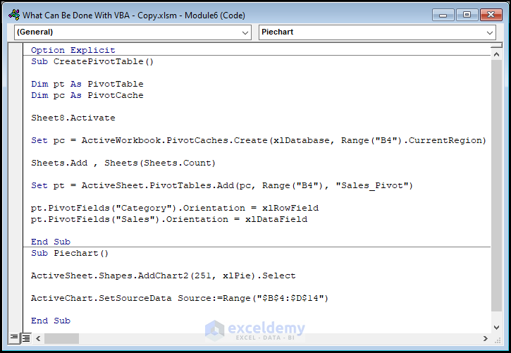
⚡ Code Breakdown:
- Enter a name for the sub-routine and define the variables.
- Activate Sheet8 using the Activate method and assign memory cache using the PivotCache object.
- Insert the PivotTable in a new sheet with the Add method.
- Position it in the preferred (B4) cell and enter the name Sales_Pivot.
- Add the Pivot Fieldse. the Category in the RowField and Sales in the DataField.
- A new sub-routine is used to insert the chart.
- Utilize the ActiveSheet property and the AddChart2 method to insert a Pie Chart.
- Employ the SourceData property to select the data range for the Pie Chart.
- Press the F5 key to run the CreatePivotTable () sub-routine.
- Execute the Piechart () sub-routine.
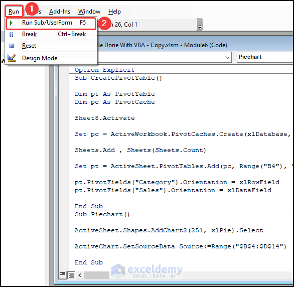
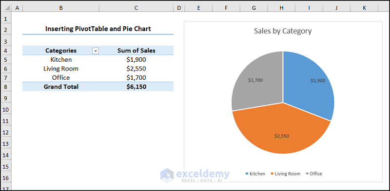
A pivot table and pie chart will be inserted in the worksheet.
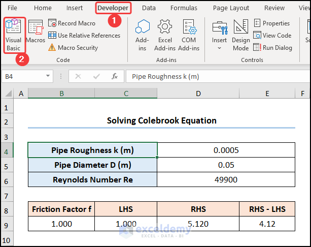
Task 4 – Solving Complex Equations
Steps:
- Go to the Developer tab and open the Visual Basic editor.
- Enter the following code into the window.
Sub Solve_Colebrook()

Static Computing As Boolean
If Round(Range("E9").Value, 3) <> 0 And Not Computing Then
    Computing = True
    Range("B9").Value = 0.01
    Range("E9").GoalSeek goal:=0, ChangingCell:=Range("B9")
    Computing = False
End If

End Sub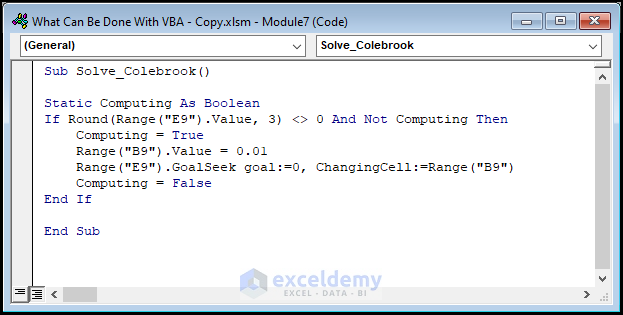
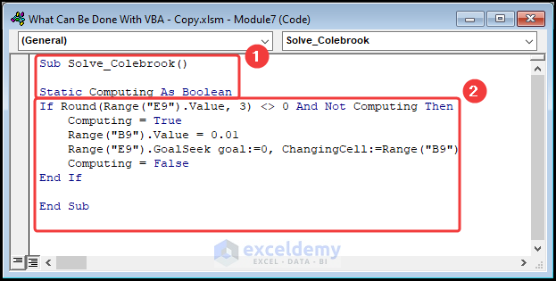
⚡ Code Breakdown:
- The sub-routine is given a name, here it is Solve_Colebrook().
- Define the variable Computing and assign Boolean data type.
- Use the If statement to check if the value in the E9 cell is not equal to zero and not equal to Computing.
- Set the value in the B9 cell to 01 using the Range object.
- Apply the Goal Seek method to determine the value of the B9 cell (Friction factor) which gives zero in the E9 (RHS – LHS) cell.
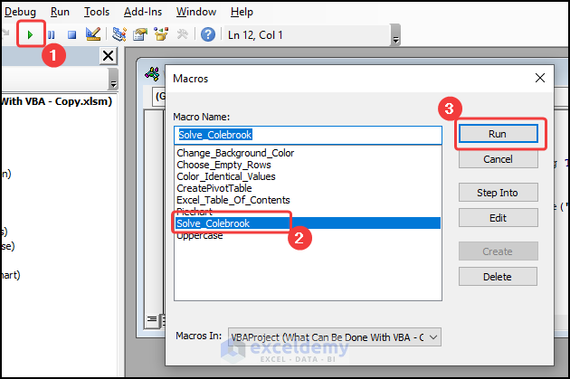
- Press the F5 key >> choose Solve_Colebrook macro >> click on Run.
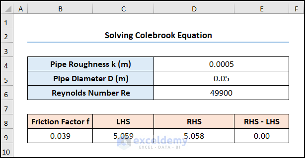
The output should look like the screenshot below.
Method 5 – Developing New Custom Functions
Steps:
- Go to the Developer tab and navigate to Visual Basic.
Enter the following code.
Function WordCount(rng As Range) As Integer
WordCount = UBound(Split(rng.Value, " "), 1) + 1
End Function
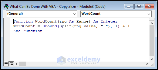
The WordCount function combines the Split and the UBound functions to find the white space character, count each word and returns the total word count.
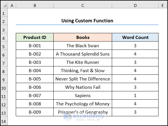
- Enter the function WordCount which takes one argument. In this case, the C5 cell refers to the text The Black Swan.
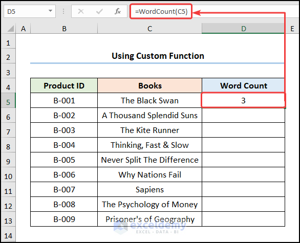
The word count of each cell will be displayed.
Method 6 – Highlighting Cell Based on a Condition
6.1 Identifying Cells with Duplicate Values
Steps:
- Go to the Developer tab and move to the Visual Basic editor.
- Insert a Module and enter the following code.
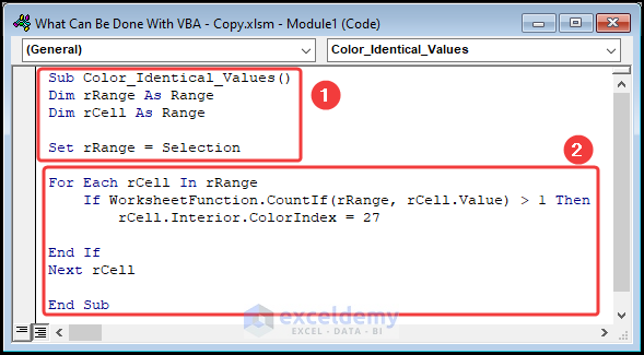
Sub Color_Identical_Values()
Dim rRange As Range
Dim rCell As Range

Set rRange = Selection

For Each rCell In rRange
    If WorksheetFunction.CountIf(rRange, rCell.Value) > 1 Then
        rCell.Interior.ColorIndex = 27

End If
Next rCell

End Sub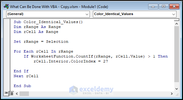
⚡ Code Breakdown:
- The sub-routine is given a name, here it is Color_Identical_Values().
- Define the variables rRange and rCell Then, set the Selection property to rRange variable.
- Use the For-If statement to loop through the values in the cell are identical. If the condition holds then use the ColorIndex property to change the cell color. Otherwise, keep the cell color unchanged.
- Close the VBA window >> select the B5:B14 cells >> click Macros.
- Select the Color_Identical_Values macro >> click on Run.
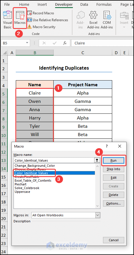
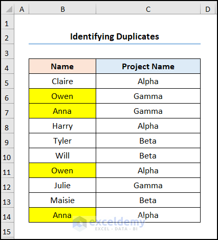
It will highlight all duplicate cells.
6.2 Changing Cell Color Based on Value
Steps:
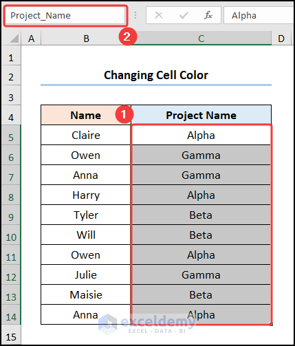
- Select the range of cells C5:C14 >> go to the Name Box, and enter in a name. We have chosen Project_Name.
- Open the Visual Basic editor and enter the following code inside the Module.
Sub Change_Background_Color()

Dim cell_value As Range
Dim project As String
Dim rng As Range

Set rng = Range("Project_Name")

For Each cell_value In rng

project = cell_value.Value
Select Case project

    Case "Alpha"
    cell_value.Interior.Color = RGB(0, 255, 0)

    Case "Gamma"
    cell_value.Interior.Color = RGB(255, 255, 0)

    Case "Beta"
    cell_value.Interior.Color = RGB(255, 0, 0)

End Select

Next cell_value

End Sub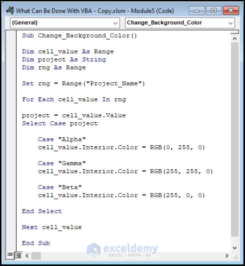
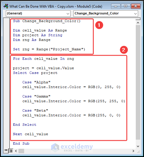
⚡ Code Breakdown:
- The sub-routine is given a name.
- Define the variable cell_value, project, and rng.
- Assign a Range and String data type to each variable.
- Insert the Named Range object in the rng variable.
- In the latter part use the For Loop statement and the Select Case statement to iterate through each of the three cases Alpha, Gamma, and Beta.
- Use the Color property to change the background color of the cells. Here, the RGB (0, 255, 0) is the Green color, the RGB (255, 255, 0) is the Yellow color, and RGB (255, 0, 0) indicates the Red color.
- Close the VBA window and press the Macros option >> choose the Change_Background_Color macro >> click on Run.
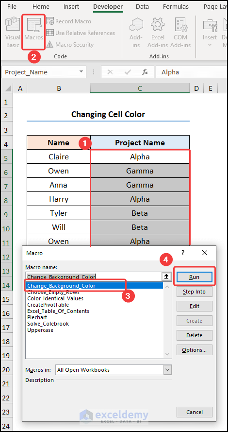
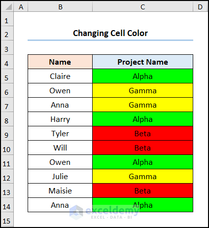
The cell color will change according to each Project Name.
Download Practice Workbook


Can you please provide me complete VBA videos?