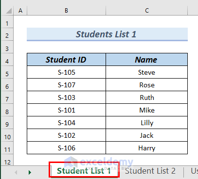
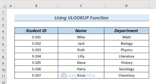
The following dataset has the Student ID and Name columns. The Student IDs are in irregular order.
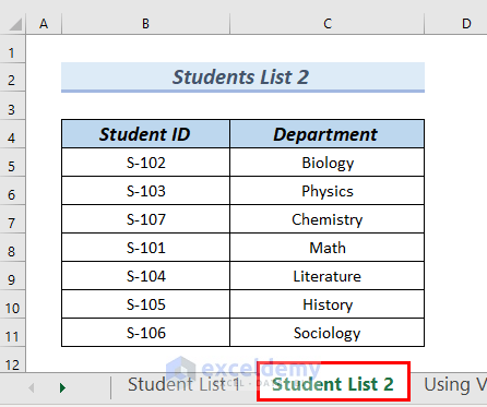
The second dataset has the Student ID and Department columns. The Student ID is also in irregular order.
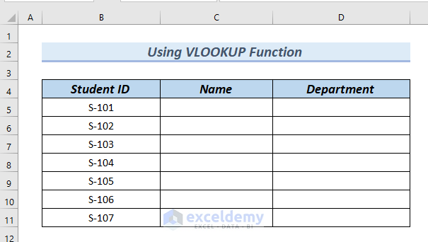
We will use the VLOOKUP function to merge two sheets into the following new Excel sheet.
Step 1: Inserting Data from the First Sheet
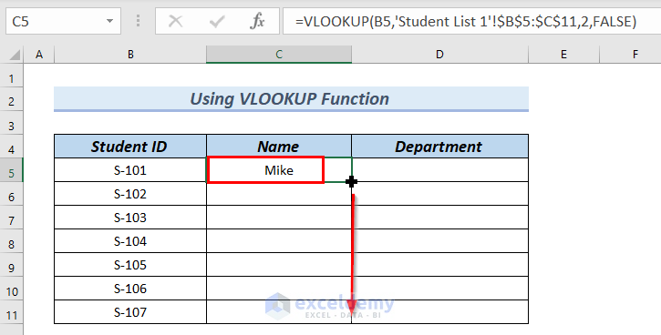
- Enter the following formula in cell C5:
=VLOOKUP(B5,'Student List 1'!$B$5:$C$11,2,FALSE)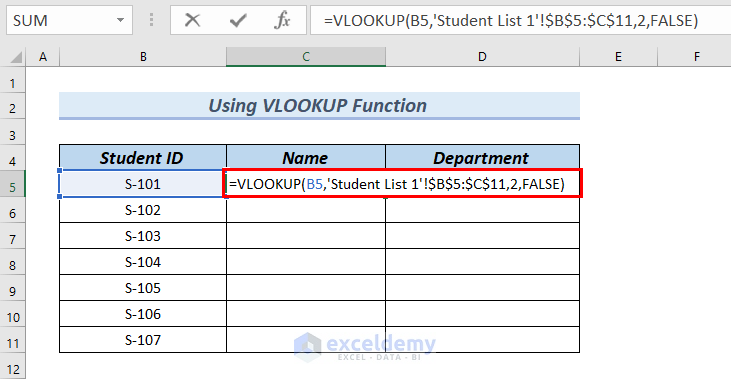
Formula Breakdown
- VLOOKUP(B5,’Student List 1′!$B$5:$C$11,2,FALSE) →The VLOOKUP function searches for values in a defined table array.
- B5 → is the lookup_value.
- ‘Student List 1’!$B$5:$C$11→ is the table_array, which is present in the sheet Student List 1.
- 2 → is col_index_num
- FALSE→ indicates the Exact match.
- VLOOKUP(B5,’Student List 1′!$B$5:$C$11,2,FALSE) → becomes
- Output: Mike
- Explanation: here, Mike is the Name for Student ID S-101.
- Press ENTER.
You can see the result in cell C5.
- Drag down the formula with the Fill Handle tool.
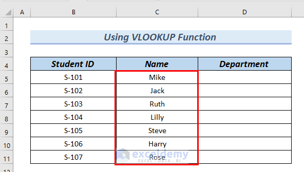
You can see the complete Name column in the new Excel sheet.
Step 2: Employing Data from the Second Sheet
- Enter the following formula in cell D5:
=VLOOKUP(B5,'Student List 2'!$B$5:$C$11,2,FALSE)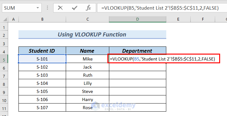
Formula Breakdown
- VLOOKUP(B5,’Student List 2′!$B$5:$C$11,2,FALSE) →The VLOOKUP function searches for values in a defined table array.
- B5 → is the lookup_value.
- ‘Student List 2’!$B$5:$C$11→ is the table_array, which is present in the sheet Student List 2.
- 2 → is col_index_num
- FALSE→ indicates the Exact match.
- VLOOKUP(B5,’Student List 2′!$B$5:$C$11,2,FALSE) → becomes
- Output: Math
- Explanation: here, Math is the Department for Student ID S-101.
- Press ENTER.
You can see the result in cell D5.
- Drag down the formula with the Fill Handle tool.
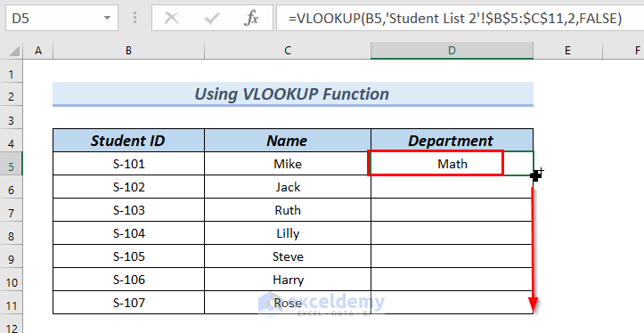
You can see the complete Department column.
- Use the VLOOKUP function to merge two Excel sheets.
How to Use the XLOOKUP Function to Merge Two Excel Sheets
Steps:
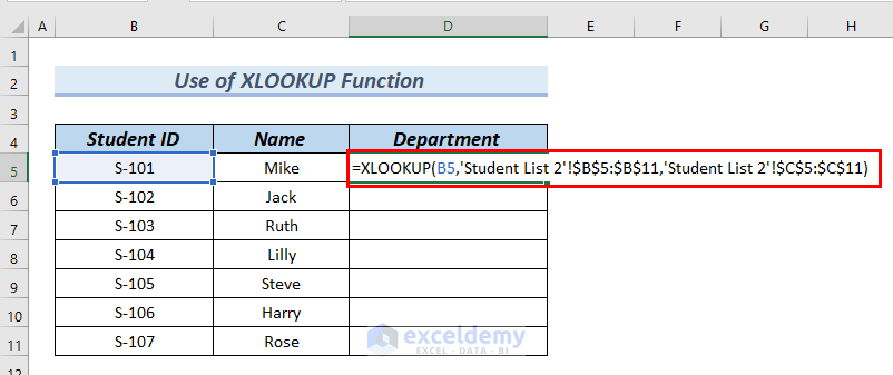
- Enter the following formula in cell C5:
=XLOOKUP(B5,'Student List 1'!$B$5:$B$11,'Student List 1'!$C$5:$C$11) 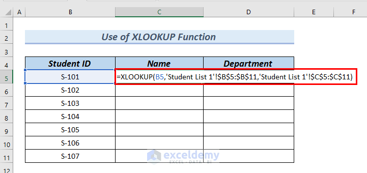
Formula Breakdown
- XLOOKUP(B5,’Student List 1′!$B$5:$B$11,’Student List 1′!$C$5:$C$11) → the XLOOKUP function searches for data or value in a table array and returns the result value in another location.
- B5 → is the lookup_value.
- ‘Student List 1’!$B$5:$B$11 → is the lookup_array.
- ‘Student List 1’!$C$5:$C$11 → is the return_array.
- XLOOKUP(B5,’Student List 1′!$B$5:$B$11,’Student List 1′!$C$5:$C$11) → becomes
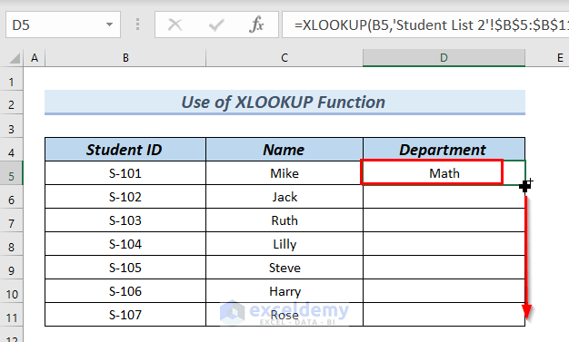
- Output: Mike
- Explanation: here, Mike is the Name for Student ID S-101
- Press ENTER.
You can see the result in cell C5.
- Drag down the formula with the Fill Handle tool.
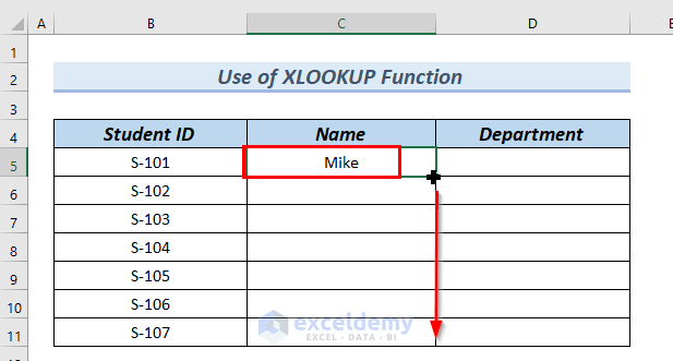
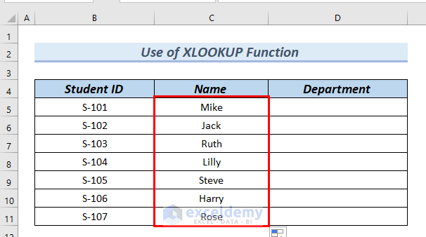
You can see the complete Name column.
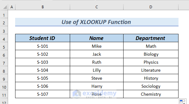
- To find the Department for the corresponding Student ID,
- Enter the following formula in cell D5:
=XLOOKUP(B5,'Student List 2'!$B$5:$B$11,'Student List 2'!$C$5:$C$11)Here, the XLOOKUP function searches for data or values in a table array and returns the result in another location.
- Press ENTER.
As a result, you can see the result in cell D5.
- Drag down the formula with the Fill Handle tool.
You can see the complete Department column.
- Use the XLOOKUP function to merge two Excel sheets.
How to Use the LOOKUP Function to Merge Two Excel Sheets
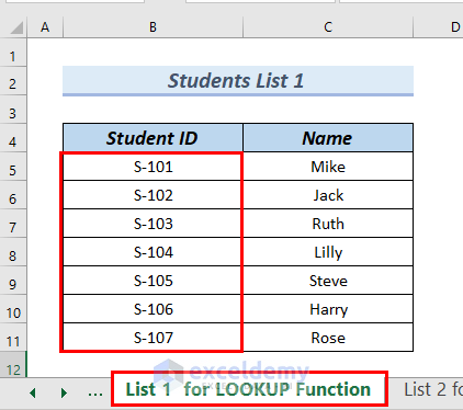
We created the Students List 1 dataset with Student ID and Name columns. It is present in List 1 for the LOOKUP Function Excel sheet. The Student ID is in regular ascending order, which is necessary when using the LOOKUP function.
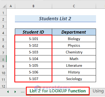
We created the Students List 2 dataset with the Student ID and Department columns. It is present in List 2 for the LOOKUP Function Excel sheet. The Student ID is in regular ascending order.
We will merge these two Excel sheets into one new sheet. The Student IDs on the new sheet are in the same order as they are in Student List 1 and Student List 2.
Steps:
- Enter the following formula in cell C5:
=LOOKUP(B5,'List 1 for LOOKUP Function'!$B$5:$B$11,'List 1 for LOOKUP Function'!$C$5:$C$11)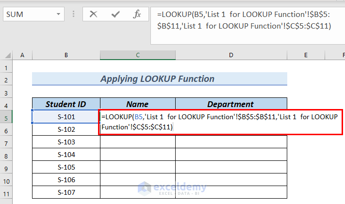
Formula Breakdown
- LOOKUP(B5,’List 1 for LOOKUP Function’!$B$5:$B$11,’List 1 for LOOKUP Function’!$C$5:$C$11) → the LOOKUP function searches for a value in a single row or single column and returns the value to another location.
- B5→ is the lookup_value.
- ‘List 1 for LOOKUP Function’!$B$5:$B$11 → is the lookup_vector.
- ‘List 1 for LOOKUP Function’!$C$5:$C$11 → is the resul_vextor.
- LOOKUP(B5,’List 1 for LOOKUP Function’!$B$5:$B$11,’List 1 for LOOKUP Function’!$C$5:$C$11) →becomes
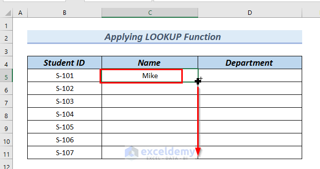
- Output: Mike
- Explanation: Here, Mike is the Name for Student ID S-101.
- Press ENTER.
You can see the result in cell C5.
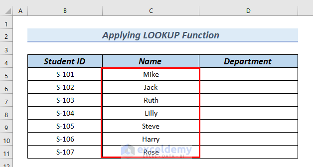
- Drag down the formula with the Fill Handle tool.
You can see the complete Name column in the new Excel sheet.
- To find the Department for the corresponding Student ID,
- enter the following formula in cell D5:
=LOOKUP(B5,'List 2 for LOOKUP Function'!$B$5:$B$11,'List 2 for LOOKUP Function'!$C$5:$C$11)Here, the LOOKUP function searches for a value in a single row or column and returns it to another location.
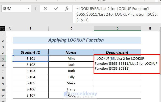
- Press ENTER.
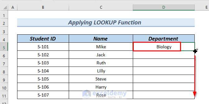
As a result, you can see the result in cell C5.
- Drag down the formula with the Fill Handle tool.
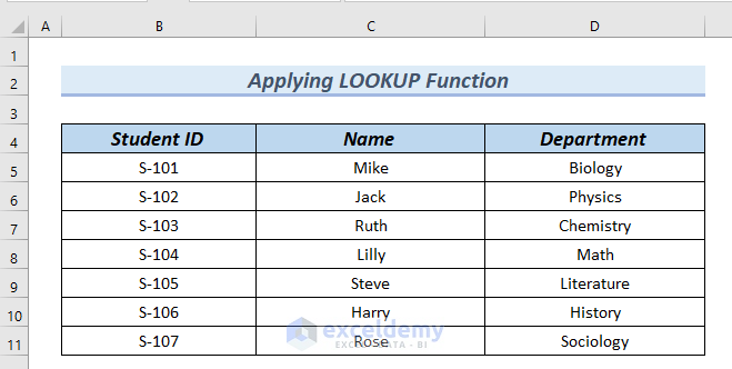
You can see the complete Department column.
- Use the LOOKUP function to merge two Excel sheets.
Things to Remember
- While using the VLOOKUP function, you must keep the Student ID column as the first column in the lookup_array
- Make sure to set FALSE in the VLOOKUP function; this will return an Exact match.
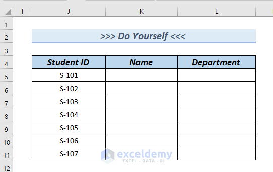
Practice Section
You can download the above Excel file to practice the explained methods.
Download the Practice Workbook
You can download the Excel file and practice.
<< Go Back To Merge Sheets in Excel | Merge in Excel | Learn Excel
Get FREE Advanced Excel Exercises with Solutions!
