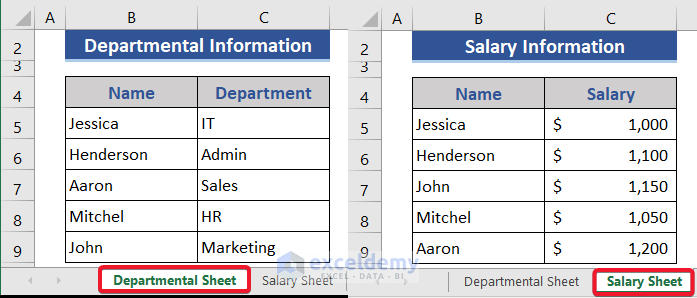
We have the salary and departmental information of some people on two different sheets. Here, we will show 3 ways to merge two sheets based on one column.
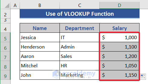
Method 1 – Using the VLOOKUP Function to Merge Two Excel Sheets Based on One Column
Steps:
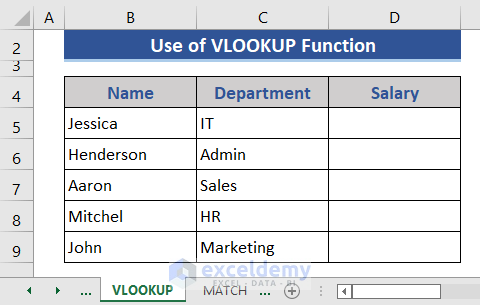
- Copy the Departmental Sheet and name it VLOOKUP.
- Create a new column named Salary in column D.
- Go to Cell D5.
- Put the following formula:
=VLOOKUP(B5,'Salary Sheet'!$B$5:$C$9,2,FALSE)
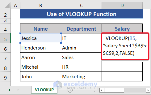
- Press the Enter button.
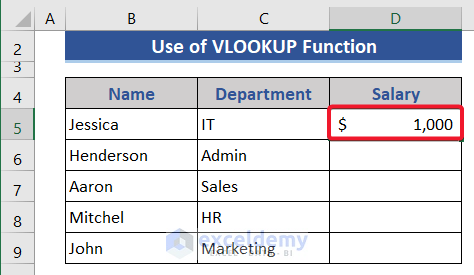
- Drag the Fill Handle icon down to get the result of the full list.
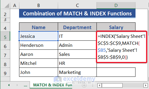
Method 2 – Combining MATCH and INDEX Functions to Merge Two Sheets in Excel
Steps:
- Create a new joined table similar to Method 1.
- Go to Cell D5 and put the formula based on the MATCH and INDEX functions.
=INDEX(‘Salary Sheet’!$C$5:$C$9,MATCH($B5,’Salary Sheet’!$B$5:$B$9,0))
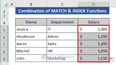
- Press Enter and pull the Fill Handle icon down to get the full result.
Formula Explanation:
- MATCH($B5,’Salary Sheet’!$B$5:$B$9,0)
The MATCH function shows the position of Cell B5 in the Range B5:B9.
Result: 1
- INDEX(‘Salary Sheet’!$C$5:$C$9,MATCH($B5,’Salary Sheet’!$B$5:$B$9,0))
The INDEX function returns the relative data of the showing position from the Range C5:C9 of the Salary Sheet.
Result: 1000
Method 3 – Merge Two Sheets Based on One Column Using Excel Power Query
Steps:
- Open a new Excel file.
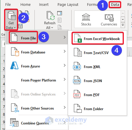
- Click on the Data tab first.
- Choose the Get Data option.
- Select File and Excel Workbook.
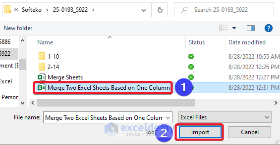
- We chose our Excel file from the File Manager.
- Click on the Import button.
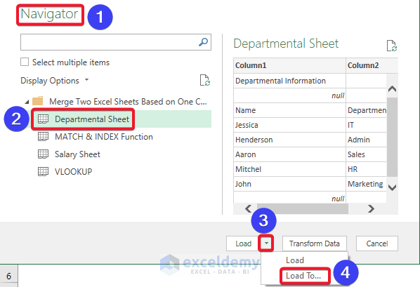
- The Navigator window appears.
- Choose one of the sheets to merge.
- Look at the bottom section.
- Press the down arrow of the Load option.
- Choose the Load to option from there.
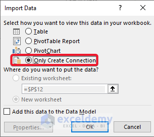
- The Import Data window appears.
- Tick the Only Create Connection option.
- Press OK.
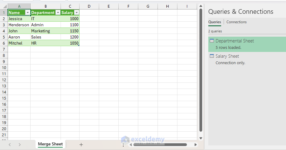
- Look at the Queries & Connections section.
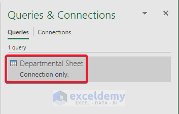
- We can see that the selected sheet has been added.
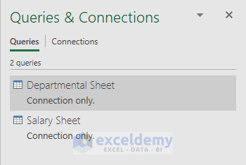
- Add the Salary Sheet in the power query.
- Double-click on the Departmental Sheet and enter the power query window.
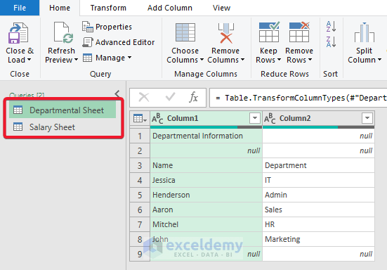
- Choose Merge Queries from the main tab.

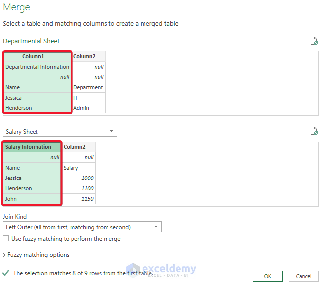
- The Merge window appears.
- We chose our second sheet from the list.
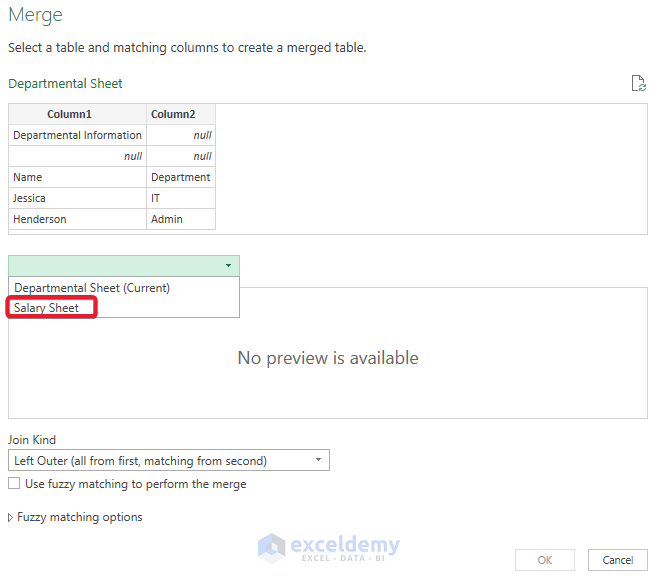
- Select the column from both sheets.
- Press the OK button.
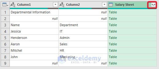
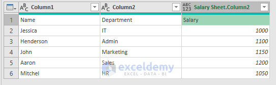
- We can see that three columns are showing.
- Click on the right upper section of the Salary Sheet column.
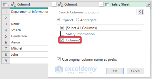
- Mark the Column2 option.
- Press the OK button.
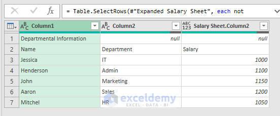
- All values are showing.
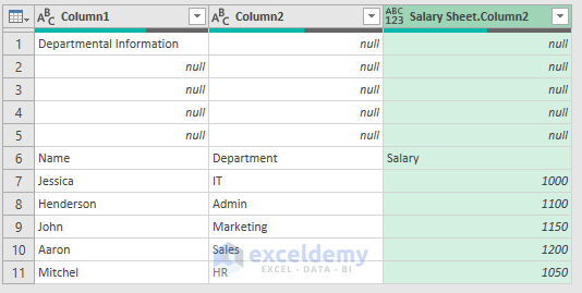
- Click on the Reduce Rows tab.
- Choose Remove Blank Rows from the Remove Rows.
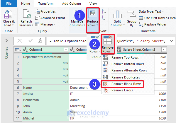
- We can see all blank rows are removed. Still, there is an unnecessary row that exists.
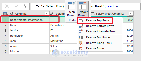
- Click on the Remove Top Rows option from the Remove Rows tab.
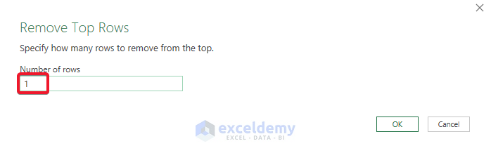
- A dialog box appears to put the number of rows. We input 1 on the box.
- Press the OK button.
- All unnecessary rows have been removed.
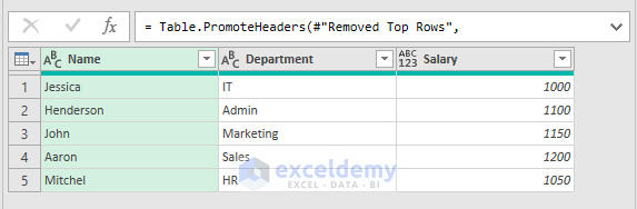
- Choose the Use First Row as Headers option.
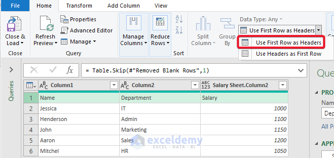
- Here’s the result.
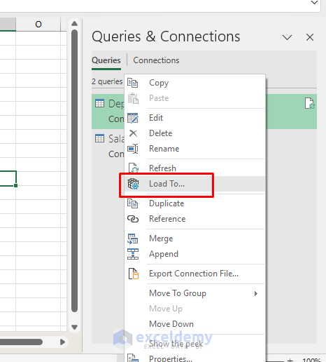
If you want to Load the table into an Excel worksheet follow these steps:
- Select the sheet name (Departmental Sheet) and Right-Click on the sheet. Then, select Load To.
- Import Data dialog box will pop up
- From there select Table.
- Then select the location where you want to put the data. Here, selected A1 cell.

Finally, data is exported to a table.
Download the Practice Workbook
<< Go Back To Merge Sheets in Excel | Merge in Excel | Learn Excel
Get FREE Advanced Excel Exercises with Solutions!

how to export the table if we are using the third step
Hello Muskan Gadodia,
To Load/Export the table into an Excel worksheet follow these steps:
Select the sheet name (Departmental Sheet) and Right-Click on the sheet. Then, select Load To.
Import Data dialog box will pop up
From there select Table.
Then select the location where you want to put the data. Here, selected A1 cell.
Finally, data is exported to a table.
You will get the steps in our updated article also.
Regards
ExcelDemy