How to Combine Rows from Multiple Sheets in Excel (4 Methods)

Method 1 – Use Consolidate Option to Combine Rows from Multiple Excel Sheets

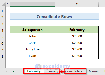
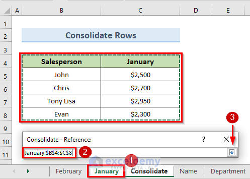
The Consolidate feature is the quickest way to combine rows. But we can only combine numeric values with this feature. In the following image, we have a dataset of salespeople and their sales amounts for the months of January and February in two different sheets. We will combine the rows of these two sheets in a new sheet named Consolidate.

STEPS:

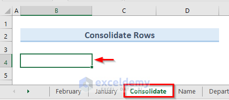
• Go to the sheet Consolidate. Select cell B4.

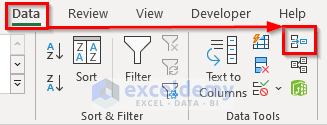
• Go to the Data tab and select the option Consolidate from the section ‘Data Tools’.

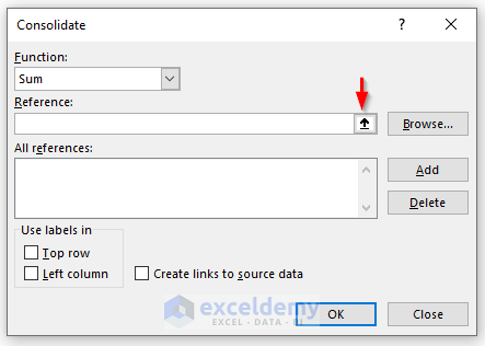
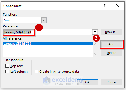
• In the Consolidate dialog box, select the SUM function. You can use any one of the available functions to consolidate your data.
• Click on the ‘Collapse Dialog Icon’ in the reference box.

• An input box like this will pop up.

• Click on the sheet January. Select the range (B4:C8) and click on the ‘Collapse Dialogue Icon’.

• This will input the selected range in the reference box.
• Click on Add to input the range in the ‘All references’ box.

• Similarly, add the range of sheet February.
• Check the box of ‘Top row’ and ‘Left column‘. Click on OK.

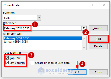
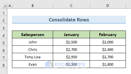
• The above command combines rows from sheets January and February in the third sheet named Consolidate.

Method 2 – Using VBA to Combine Rows from Multiple Sheets in Excel

In order to combine rows from multiple sheets in Excel more dynamically, you can use VBA (Visual Basics for Applications) code.

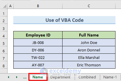
In the first image, we have a sheet named Department that contains ‘Employee ID’ and their ‘Full Name’.

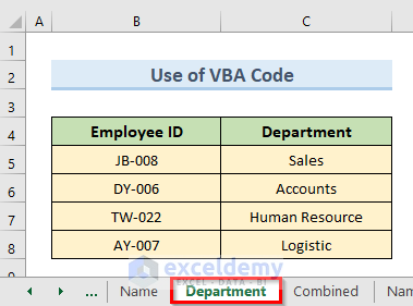
In the second image, we have a sheet named Department that consists of ‘Employee ID’ and their working Department.

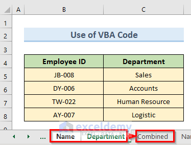
We will combine the rows of these two datasets with VBA code.

STEPS:

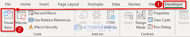
• Go to the Developer tab and select the option ‘Visual Basic’.

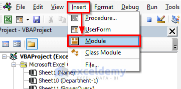
• In the dialog box, go to the Insert tab and select the option Module.

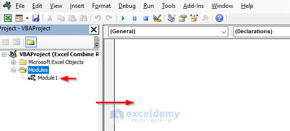
• This will insert a module named ‘Module 1’. Click on ‘Module 1’ and we will get a blank VBA module.

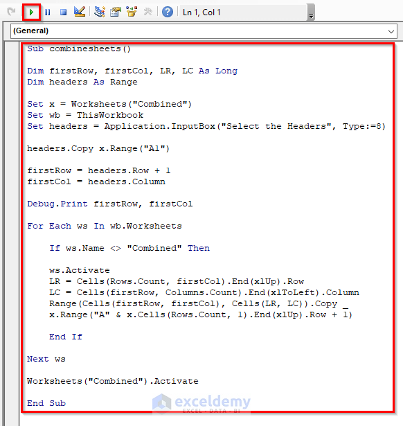
• Enter the following code in the blank module:

Sub combinesheets()
Dim firstRow, firstCol, LR, LC As Long
Dim headers As Range
Set x = Worksheets("Combined")
Set wb = ThisWorkbook
Set headers = Application.InputBox("Select the Headers", Type:=8)
headers.Copy x.Range("A1")
firstRow = headers.Row + 1
firstCol = headers.Column
Debug.Print firstRow, firstCol
For Each ws In wb.Worksheets
If ws.Name <> "Combined" Then
ws.Activate
LR = Cells(Rows.Count, firstCol).End(xlUp).Row
LC = Cells(firstRow, Columns.Count).End(xlToLeft).Column
Range(Cells(firstRow, firstCol), Cells(LR, LC)).Copy _
x.Range("A" & x.Cells(Rows.Count, 1).End(xlUp).Row + 1)
End If
Next ws
Worksheets("Combined").Activate
End Sub

• Click on Run or press the F5 to run the code.

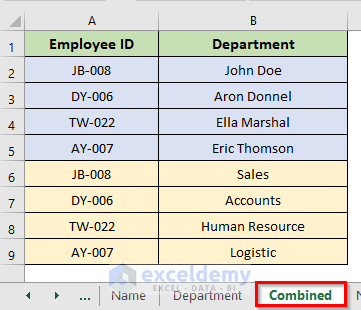
• This will combine the rows of the two sheets that we have selected in a new sheet named Combined.

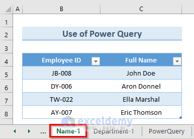
Method 3 – Using Excel Power Query to Combine Rows from Multiple Sheets

Excel’s ‘Power Query’ is a powerful tool for combining and analyzing data.

When using ‘Power Query’ to combine data from different sheets, the data must be in an ‘Excel Table’ format or at least in named ranges.

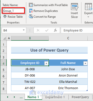
In the first image, we have the dataset of sheet ‘Name-1’ which is in table format.

Select any cell from the table. Go to the ‘Table Design’ tab and rename the table to ‘Group-1’.

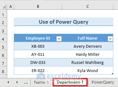
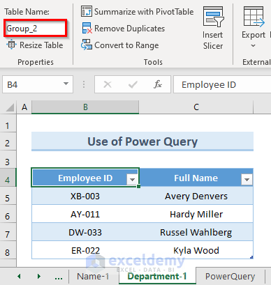
In the second image, we have the dataset of sheet ‘Department-1’ which is also in table format.

Select any cell from the table. Go to the ‘Table Design’ tab and rename the table to ‘Group-2’.

STEPS:

• Go to Data > Get Data > From Other Sources > Blank Query.

• A new window named ‘Power Query Editor’ will pop up.
• Enter the following formula in the formula bar:

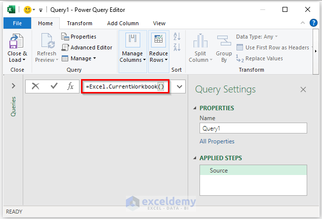
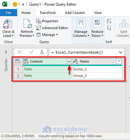
• Press Enter. This will display the names of all the tables in the entire workbook.
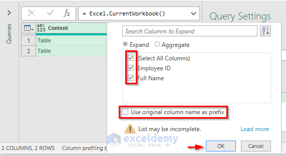
• Click on the double-pointed arrow from the content header cell.

• From the options, check the columns that you want to combine.
• Uncheck the option ‘Use original column name as prefix’.
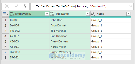
• Click on OK.

• The above command will combine the rows of the sheets which we have selected.

Loading Combined Data to Another Worksheet

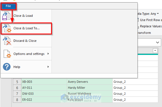
• Go to the File
• Select the option ‘Close & Load To’.

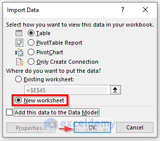
• In the dialog box, check the option ‘New worksheet’.
• Click on OK.

• The above action will load the combined rows in a new sheet named ‘Query 1’.

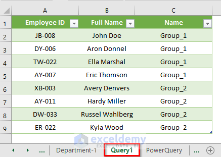
Notes: If we follow the above method to combine rows from multiple sheets, we might face a problem. Look at the following image. Our query table named ‘Query1’ consists of 9 rows including the headers.

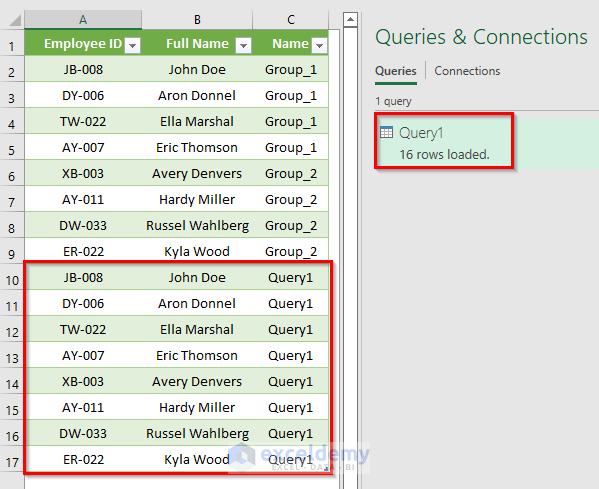
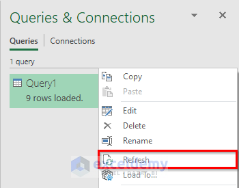
Right-click on the table name and refresh it.

We can see that the loaded row numbers have changed to 16 from 9. This is because the data from our new table ‘Query1’ will be added every time we refresh.

In order not to change the row number with each refresh,

STEPS:

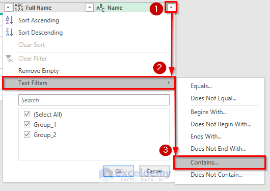
• Click on the drop-down of the header cell ‘Name’.
• Hover the cursor on the option ‘Text Filters’
• Select the option Contains.

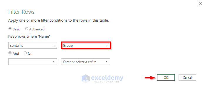
• A new dialogue box will appear. In the field text of the Contains option insert the value, Group.
• Click on OK.

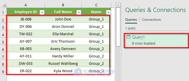
• Refresh the table.

• You will notice that no new rows will be loaded with refresh. The loaded row number will show 8 because this time, we are only calculating rows that contain the value Group. So, the header row doesn’t come into consideration.

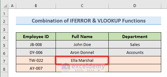
Method 4 – Joining IFERROR and VLOOKUP Functions to Combine Rows

The IFERROR function delivers a value you provide; if a formula calculates to an error, otherwise, it provides the formula’s result.

The VLOOKUP function allows you to look up data in a vertically structured table.

The first image, we have the dataset of the sheet named ‘Name (2)’.

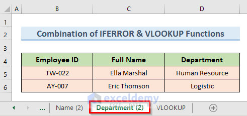
In the second image, we have the dataset of the sheet named ‘Department (2)’.

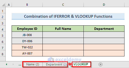
We will combine the rows of sheets ‘Name (2)’ and ‘Department (2)’ in a new sheet named VLOOKUP.

STEPS:

• Enter the following formula in cell C5:

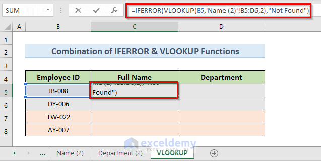
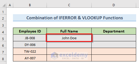
• Press Enter. We can see the value of cell C5 of the sheet ‘Name (2)’ in our selected cell.

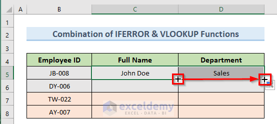
• Select cell C5. Move the mouse cursor to the bottom right corner of the selected cell so that it turns into a plus (+) sign like the following image.
• Click on the plus (+) sign and drag the Fill Handle horizontally to cell D10 to copy the formula of cell C5 in other cells. We can also double-click on the plus (+) sign to get the same result.

• If we drag the Fill Handle tool from D5 to D10, we will get all the row values of sheet ‘Name (2)’ in our new sheet.

• If we drag the Fill Handle tool one step down, it will give us the value ‘Not Found’. This is because there is no employee with the corresponding ‘Employee ID’ in the ‘Name (2)’ sheet.

• Select cell C7 and enter the following formula:

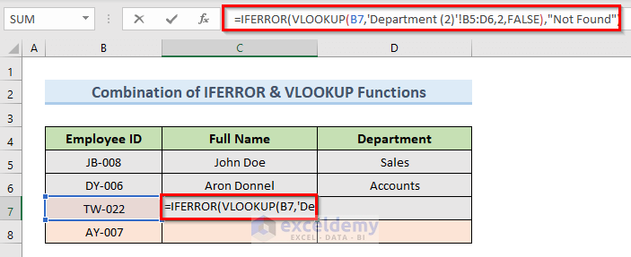
• Press Enter. We can see the ‘Full Name’ in cell C7.

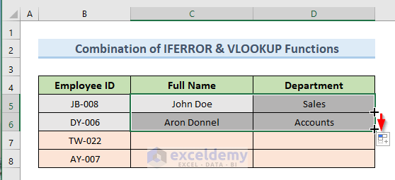
• Drag the Fill Handle tool horizontally from cell C5 to D5.

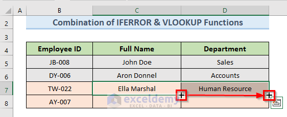
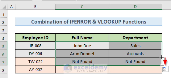
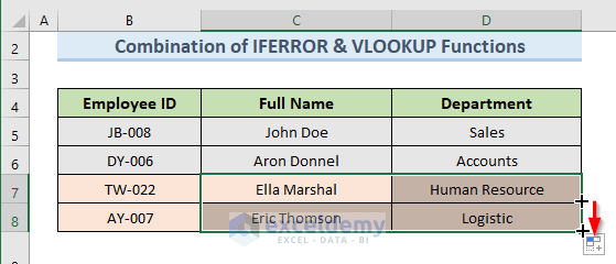
• Drag the Fill Handle tool from cell D7 to D8. This action will combine the rows of sheet ‘Department (2)’ with the rows of the sheet ‘Name (2)’ in the new sheet named VLOOKUP.

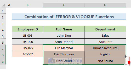
• If we drag the Fill Handle tool one more step down, we will get the value ‘Not Found’. This is because the value with the corresponding ‘Employee ID’ is not found in the sheet named ‘Department (2)’.

How Does the Formula Work?

• VLOOKUP(B5,’Name (2)’!B5:D6,2): This part finds the value of cell B5 in sheet ‘Name (2)’.
• IFERROR(VLOOKUP(B5,’Name (2)’!B5:D6,2),”Not Found”): This returns the lookup value. If the value is not found, return ‘Not Found’.

Download Practice Workbook

<< Go Back To Merge Sheets in Excel | Merge in Excel | Learn Excel