The general formula to determine the upper control limit is:
UCL = Average + (3*Standard Deviation)
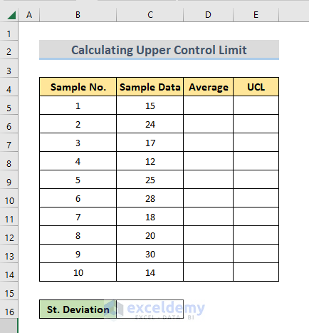
STEP 1- Enter Sample Data to calculate the Upper Control Limit
- Data was entered in the Sample Data column.
STEP 2 – Determine the Average of Sample Data
- Enter the following formula in D5.
=AVERAGE($C$5:$C$14)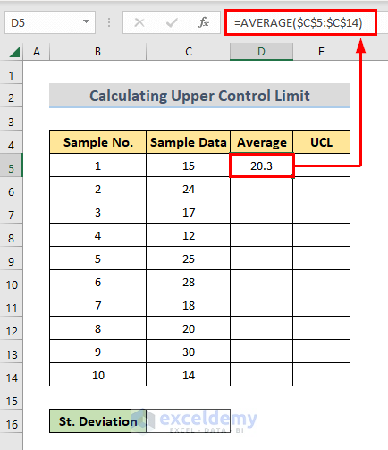
Note: A fixed cell reference was used in the formula. Press Alt + F4 to make a cell reference fixed.
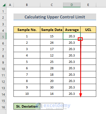
- Drag down the Fill Handle to see the result in the rest of the cells.
STEP 3 – Find the Standard Deviation
- Enter the following formula in C16.
=STDEV.S($C$5:$C$14)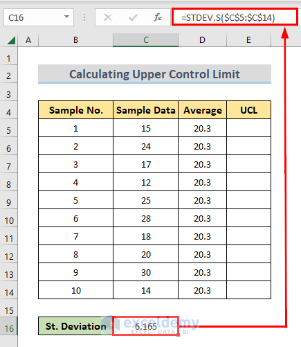
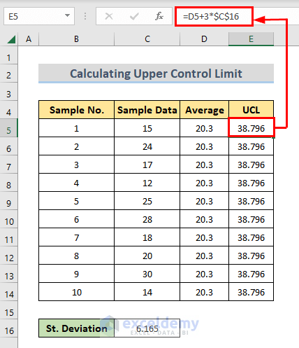
STEP 4 – Calculate the Upper Control Limit with a Formula
- Enter the following formula in E5 and press Enter.
=D5+3*$C$16- The upper control limit is displayed in E5.
- Drag down the Fill Handle to see the result in the rest of the cells.
How to Determine LCL with UCL and Create a Chart
Calculate the upper control limit following the previous steps.
- Enter the following formula in F5 to get the lower control limit.
=D5-3*$C$16- Drag down the Fill Handle to see the result in the rest of the cells.
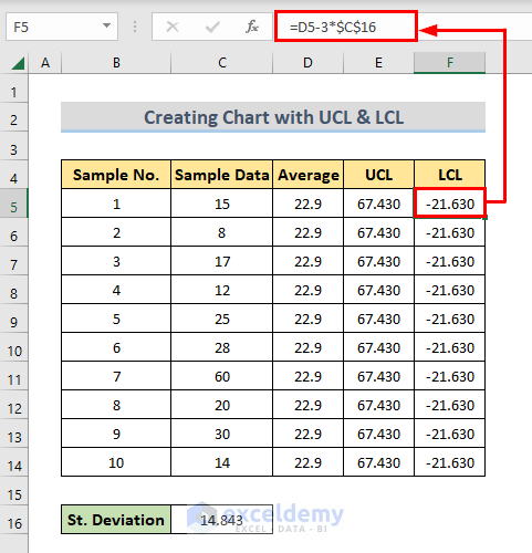
Note: In the formula for the lower control limit 3*Standard Deviation was subtracted from the Average.
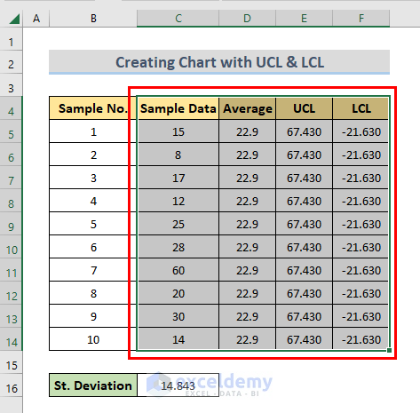
- Select the whole dataset.
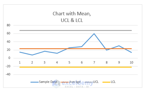
- Go to the Insert tab and select Line or Area Chart > 2-D > Line.
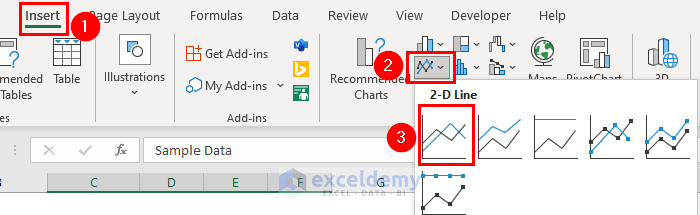
- The line chart is displayed. Name it.
- Select any data point in the line chart and right-click it.
- Select Add Data Label.
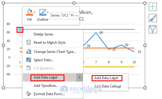
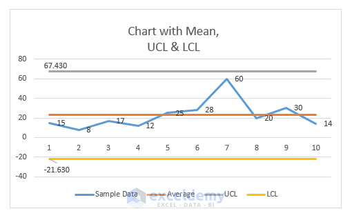
- Add other Data Labels.
Download Practice Workbook
Download the practice workbook here.
Related Articles
<< Go Back to Excel Control Chart | Excel Charts | Learn Excel
Get FREE Advanced Excel Exercises with Solutions!
