Gridlines, the horizontal and vertical gray-colored lines that differentiate between cells in a worksheet, are displayed by default in an Excel worksheet. But the gridlines disappear as soon as we apply the Fill Color feature to color the cells, which may not be desired. In this article, we will demonstrate simple yet effective methods to show gridlines after using Fill Color in Excel.
To illustrate, we will use the following sample dataset as an example. We have colored the range B4:D10 using the Fill Color feature in Excel. As a result, the gridlines have disappeared from that range.
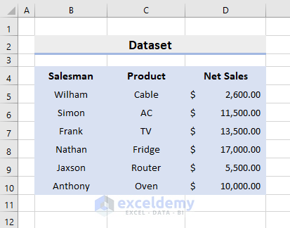
Let’s show them again.
Method 1 – Using Borders Drop-Down Feature
Steps:
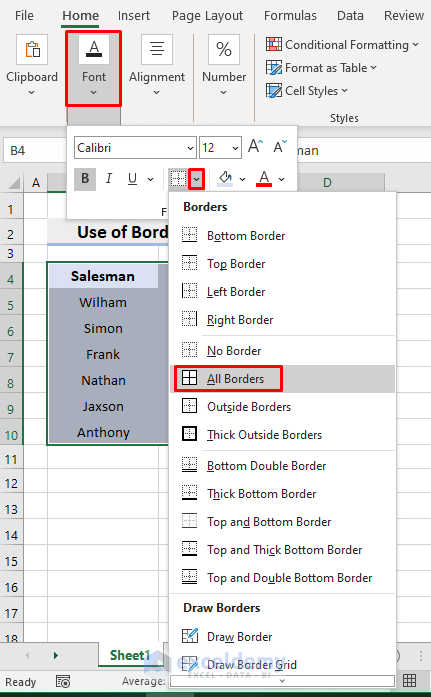
- Select the colored range B4:D10.
- Go to Home ➤ Font ➤ Borders.
- Click the Borders Drop–Down icon.
- Select All Borders.
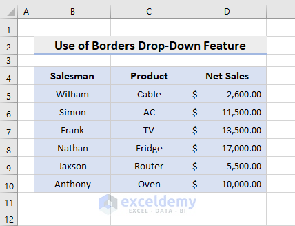
Gridlines are returned to the desired area.
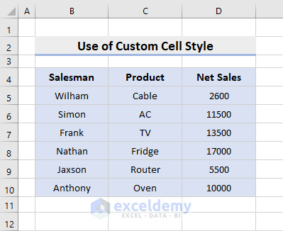
Method 2 – Using Custom Cell Style
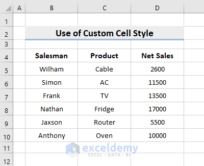
We can create a Custom Cell Style to show gridlines in a colored range of cells. In the following dataset, we will highlight the range B4:D10 in Blue color while preserving the gridlines.
Steps:
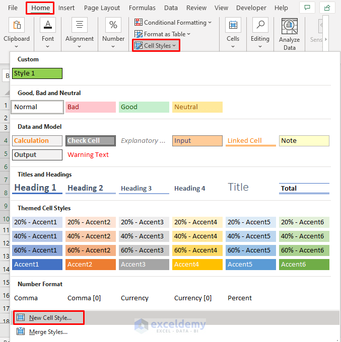
- Select Home ➤ Styles ➤ Cell Styles ➤ New Cell Style.
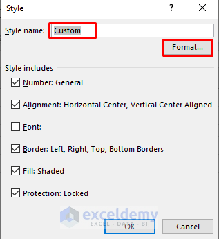
- The Style dialog box will pop out.
- Enter Custom in the Style name.
- Press Format.
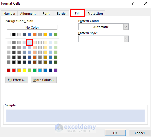
A new dialog box will emerge.
- Under the Fill tab, select the Blue color.
- Under the Border tab, select the Gray color from the Color option (to match the color of the Gridlines).
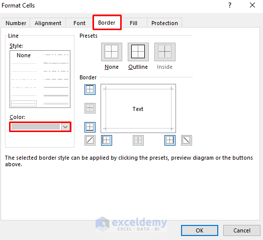
- Click OK.
The highlighted range also has gridlines.
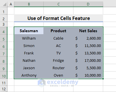
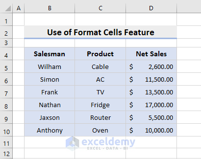
Method 3 – Using Excel Format Cells Feature
Steps:
- Select the colored range B4:D10.
- Press ‘Ctrl’ and ‘1’ simultaneously.
The Format Cells dialog box will appear.
- Go to the Border tab and select the Gray color in the Color field.
- Select the Outline and Inside from the Presets.
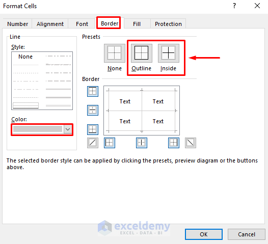
- Click OK to return the gridlines.
Read More: How to Keep Gridlines When Copy and Paste in Excel
Method 4 – Using VBA Code
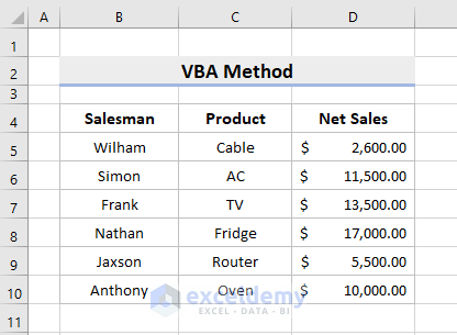
In the below dataset, we have the cell values in the range B4:D10 and we are yet to color the range. We’ll use VBA code to show Gridlines after using Fill Color.
Steps:
- Go to Developer ➤ Visual Basic.
The VBA window will appear.
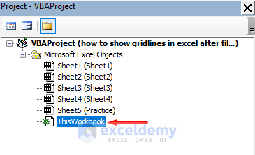
- Double-click ThisWorkbook which you’ll find in the left-most pane.
A dialog box will appear.
- Copy the following code and paste it into the box.
Dim rng As Range
Private Sub Workbook_SheetSelectionChange(ByVal Sh As Object, ByVal Target As Range)
    On Error Resume Next
    If Not rng Is Nothing Then DrawBorders rng
    Set rng = Target
End Sub
Private Sub DrawBorders(ByVal rg As Range)
    Dim cells As Range
    Application.ScreenUpdating = False
    For Each cells In rg
        If cells.Interior.ColorIndex = xlNone Then
            With cells.Borders
                If .ColorIndex = 15 Then
                    .LineStyle = xlNone
                End If
            End With
        Else
            With cells.Borders
                If .LineStyle = xlNone Then
                    .Weight = xlThin
                    .ColorIndex = 15
                End If
            End With
        End If
    Next
    Application.ScreenUpdating = True
End Sub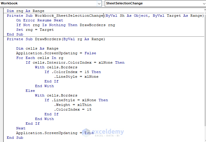
- Save the code and close the VBA window.
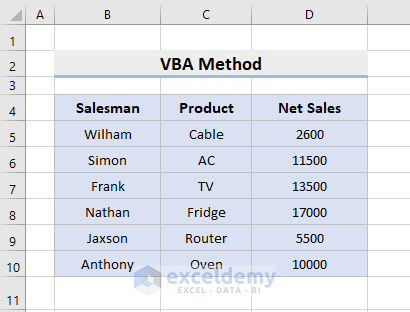
- Highlight the range B4:D10 in Blue color.
The gridlines will appear automatically.
Download Practice Workbook
Related Articles
- How Do You Fix Missing Gridlines in Excel
- How to Get Gridlines Back in Excel
- [Fixed] Excel Gridlines Not Showing by Default
<< Go Back to Show Gridlines | Gridlines | Learn Excel
Get FREE Advanced Excel Exercises with Solutions!
