How to Create a Progress Bar in Excel Cells Using Conditional Formatting

Dataset Overview

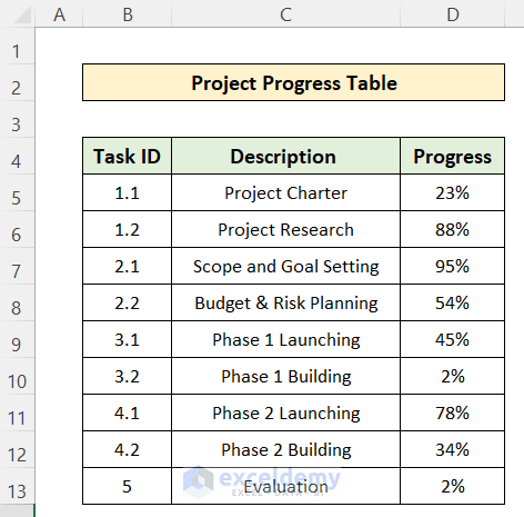
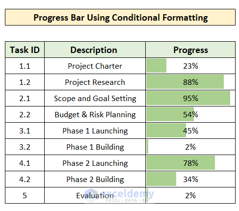
Suppose we have a dataset containing a number of tasks in a project which is running. Another column shows the percentage completed of the task. We want to make a progress bar in this column using conditional formatting.

Step 1 – Select the Progress Data and Go to Conditional Formatting

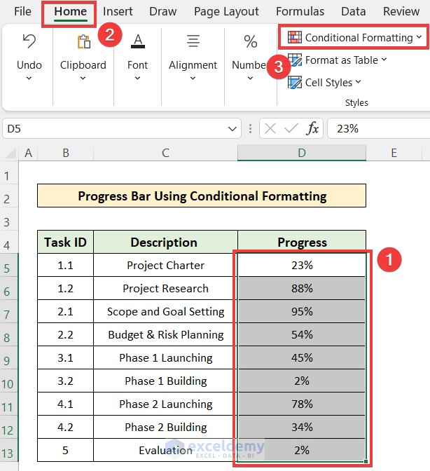
• Select the cells in the Progress column.
• Go to the Home tab and choose the Conditional Formatting feature.

Step 2 – Select More Rules from Data Bars Options

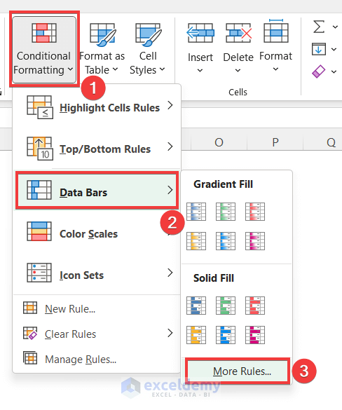
• Click on Conditional Formatting, and you’ll see additional options.
• Choose Data Bars from the list.
• Select More Rules from the sub-category.

Step 3 – Insert Formatting Rules and Apply

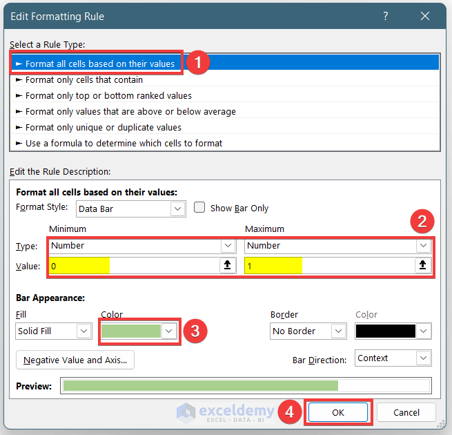
• In the Edit Formatting Rule window that appears:
  • Set the Rule Type to the first option.
  • For both the Minimum and Maximum values, select Number.
  • Insert the value = 0 for the minimum and = 1 for the maximum (since the data bar ranges from 0% to 100%).

Note: To apply the value 100%, make sure to insert 1 in the maximum value box.

• • Choose a color for the bar appearance, and you can preview it.
  • Press OK.

As a result, your progress column will display progress bars in the cells.

Download Practice Workbook

You can download the practice workbook from here:

Related Articles

• How to Create Progress Bar Based on Another Cell in Excel
• How to Show Percentage Progress Bar in Excel

<< Go Back to Data Visualisation in Excel | Learn Excel