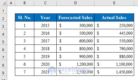
How to Create a Progress Bar in Excel (3 Easy Methods)

Suppose we have a dataset of a company’s year-wise Forecasted Sales and Actual Sales. We will create a progress bar graphing both the Forecasted Sales and Actual Sales.

Method 1 – Insert a Bar Chart to Create a Progress Bar

Steps:

Select data from your data table with the heading that you want to plot in the progress bar chart. We have selected cells (C4:E11).
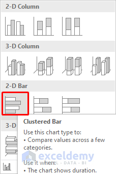
Go to the Charts list from the Insert option.

Choose a Clustered Bar from the 2-D Bar.

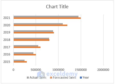
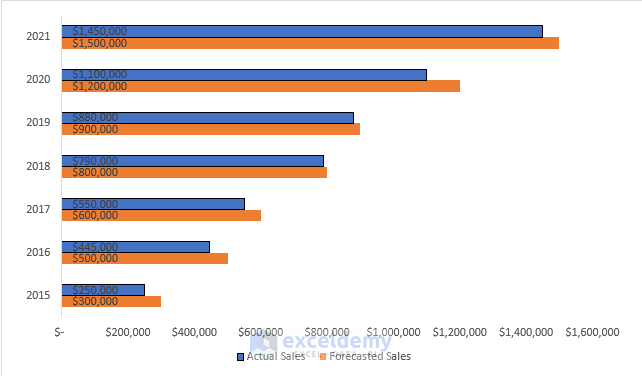
You can see a chart will be created plotting all the sales year-wise.

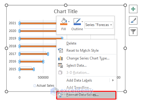
To edit the chart, select bars from the diagram and right-click on them to show options.
Choose Format Data Series.

Go to Fill and select Solid Fill.
Choose a color from the Color row and select a border color from the Border options.

Remove unnecessary data and you will get a progress bar.

Method 2 – Use Conditional Formatting to Create a Progress Bar

Steps:

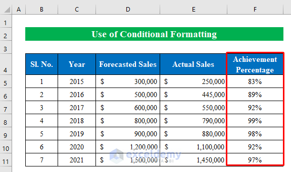
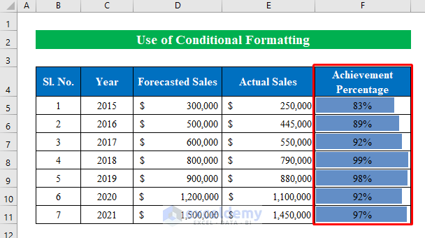
Calculate the achievement percentage by dividing the actual sales with the forecasted sales.

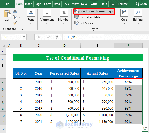
Select the column with the percentage values.
Click on Conditional Formatting from the ribbon.

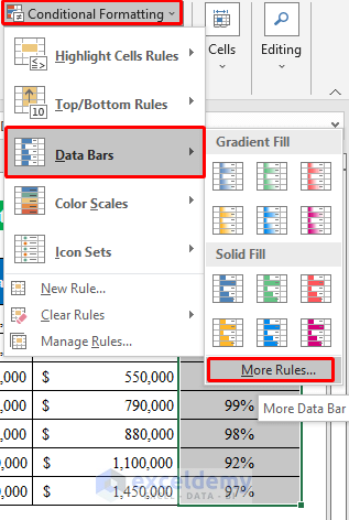
Go to More Rules from the Data Bars.

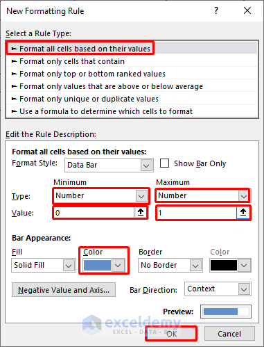
A new window will pop up named New Formatting Rule.
In Select a Rule Type, select Format all cells based on their values.
Change the type to Number in both the Minimum and Maximum sections.
Type 0 in the minimum part and 1 in the maximum part.
Choose a color for the progress bar and press OK to continue.

This creates a small progress bar for every row in Excel.

Method 3 – Use VBA Code to Create a Progress Bar

Steps:

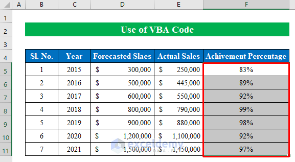
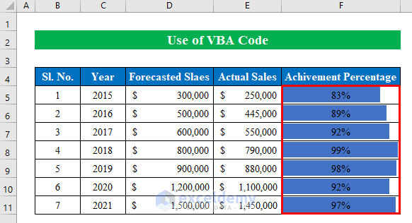
Create a column and calculate the completion percentages in it (see Method 2).
Select cells (F5:F11) to apply the code.
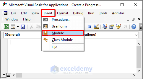
Press Alt + F11 to open the Microsoft Visual Basic for Applications window.

Create a new module from the insert option.

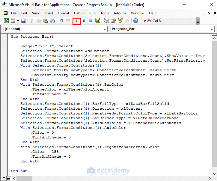
In the module, apply the following code:

Sub Progress_Bar()
Range("F5:F11").Select
Selection.FormatConditions.AddDatabar
Selection.FormatConditions(Selection.FormatConditions.Count).ShowValue = True
Selection.FormatConditions(Selection.FormatConditions.Count).SetFirstPriority
With Selection.FormatConditions(1)
.MinPoint.Modify newtype:=xlConditionValueNumber, newvalue:=0
.MaxPoint.Modify newtype:=xlConditionValueNumber, newvalue:=1
End With
With Selection.FormatConditions(1).BarColor
.ThemeColor = xlThemeColorAccent1
.TintAndShade = 0
End With
Selection.FormatConditions(1).BarFillType = xlDataBarFillSolid
Selection.FormatConditions(1).Direction = xlContext
Selection.FormatConditions(1).NegativeBarFormat.ColorType = xlDataBarColor
Selection.FormatConditions(1).BarBorder.Type = xlDataBarBorderNone
Selection.FormatConditions(1).AxisPosition = xlDataBarAxisAutomatic
With Selection.FormatConditions(1).AxisColor
.Color = 0
.TintAndShade = 0
End With
With Selection.FormatConditions(1).NegativeBarFormat.Color
.Color = 255
.TintAndShade = 0
End With
End Sub

Press Run.

This automatically creates progress bars in new cells.

Things to Remember

In Method 2, you can use different types of bar charts from the New Formatting Rule window. Open the drop-down list of Format Style to make different types of formats inside a cell.

Download Practice Workbook

Download this practice workbook to experiment with progress bars while you are reading this article.

Create a Progress Bar.xlsm

<< Go Back to Data Visualisation in Excel | Learn Excel

Get FREE Advanced Excel Exercises with Solutions!