Method 1 – Format Cells to Keep Leading Zeros in Excel
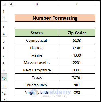
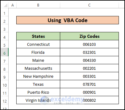
Here is a list of eight states with their Zip Codes. Several of these zip codes should begin with one or more zeros. We want to format all the zip codes by adding the necessary leading zeros.
Option 1.1 – Customize Number Format
Steps:
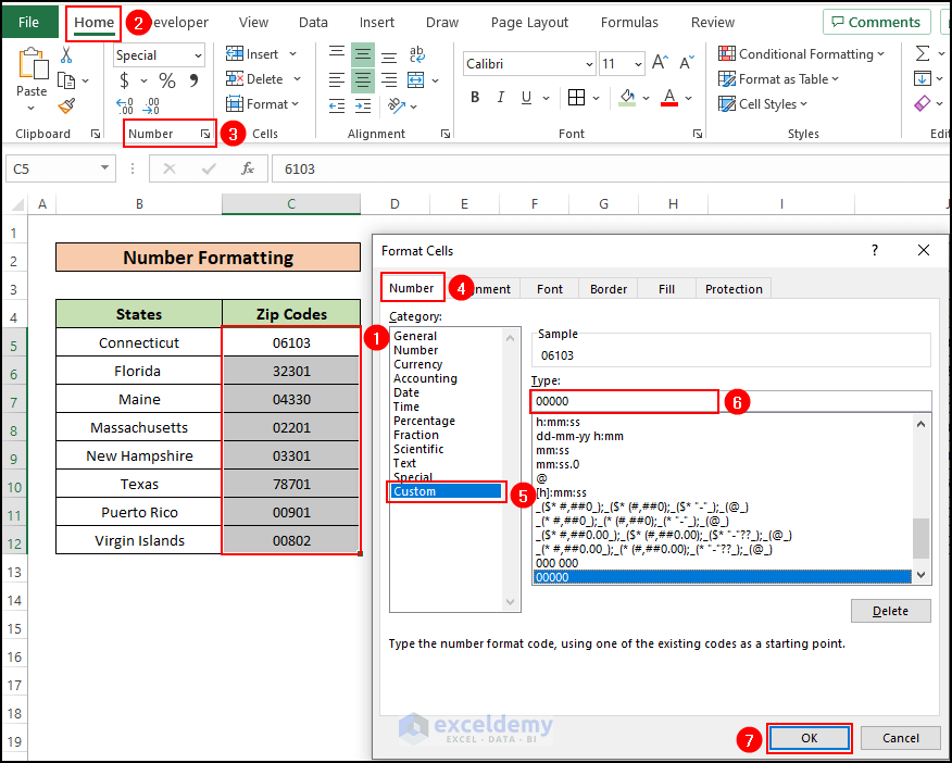
- Select all the cells (C5:C12) containing zip codes.
- Under the Home ribbon, click on the dialog box option as shown in the bottom right corner of the Number group of commands.
- Choose Custom from the list of categories in the Format Cells dialog box.
- Add 00000 in the Customized Type format box.
- Press OK.
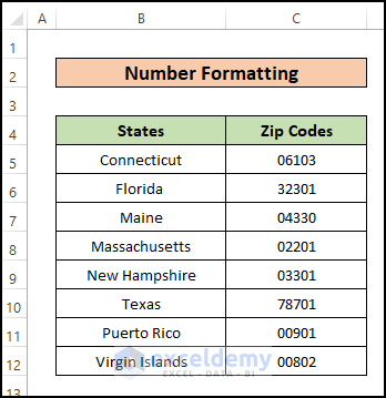
- Any necessary zeros were added so that all the zip codes have the same 5-digit format.
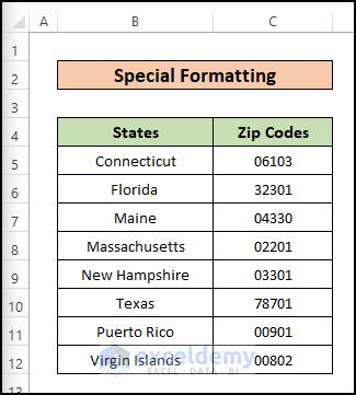
Option 1.2 – Use Built-In Special Formats
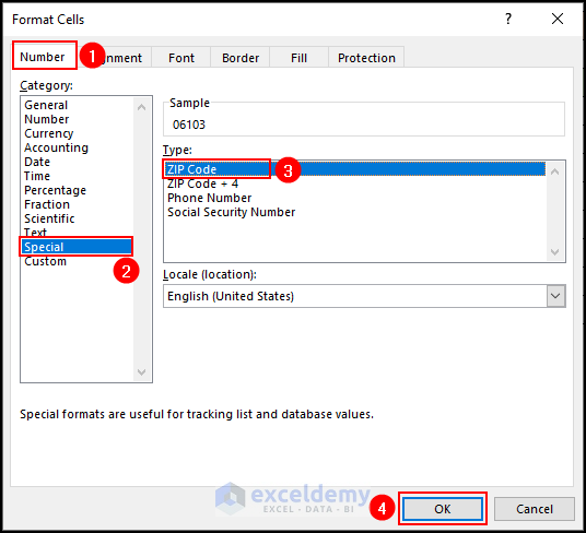
Choose the Special option from the Category list in the Format Cells dialog box. Select the type Zip Code and press OK.
- You can also use this method to keep leading zeros when working with Phone Numbers, Social Security Numbers, etc. The default location is USA. You can change the location by selecting another option from the Locale drop-down.
- Leading zeros now remain in front of the numbers where needed.
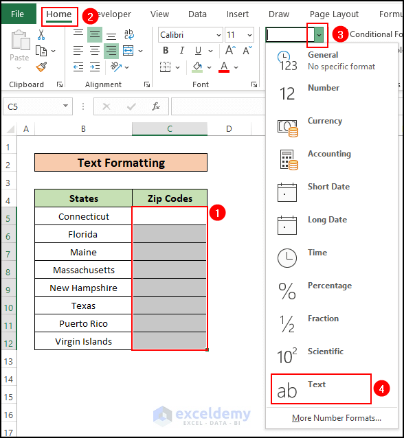
Option 1.3 – Apply Text Format
Steps:
- Select the cells where you want to input zip codes.
- From the Number group of commands, select the format Text from the drop-down menu.
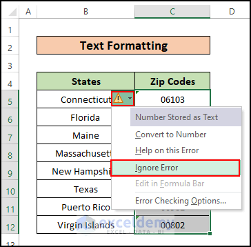
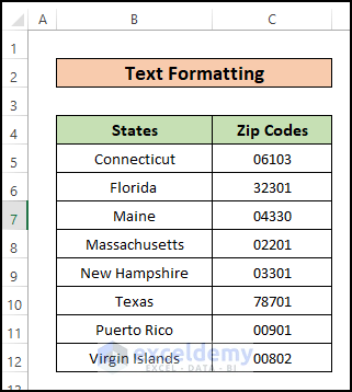
- Enter all the zip codes into the cells. You will see that no leading zeroes are removed.
- An error message saying “Number Stored as Text” will appear from a yellow drop-down option beside the cells. Select ‘Ignore Error’ for each cell.
- This method is time-consuming, so it is more effective when inputting data rather than formatting a range of pre-existing data.
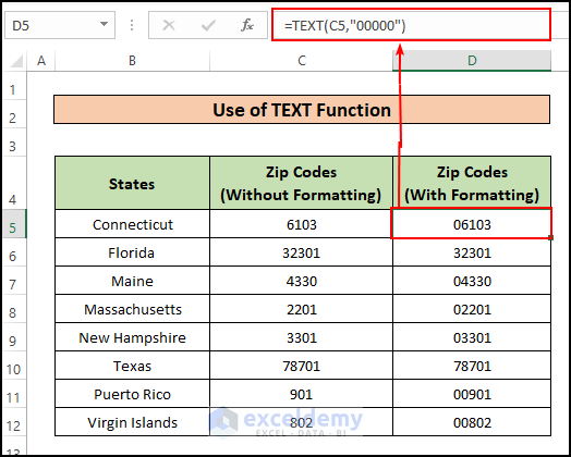
Method 2 – Use the TEXT Function to Add Preceding Zeros in Excel
Steps:
- Insert the following formula into Cell D5:
=TEXT(C5,"00000")
Formula Breakdown:
- The TEXT function converts a number to text in a specific value format.
- C5 is the cell value that is formatted in “00000” text format.
- Press Enter.
- Use the Fill Handle option from Cell D5 to format all the cells through to Cell D12.
- You will see an error warning you that you have inserted numbers as text input. Click on the error icon and select the “Ignore Error” option.
Read More: How to Keep Leading Zeros in Excel CSV
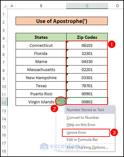
Method 3 – Add Apostrophes Before Numbers to Keep Leading Zeros in Excel
- Add an apostrophe manually before each number and then add the leading zeros.
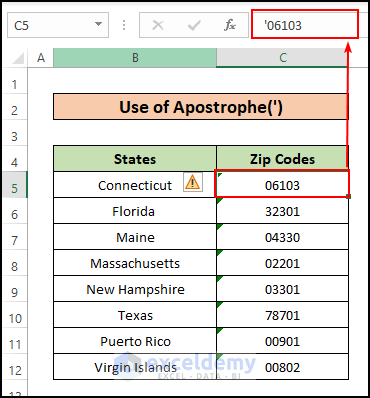
- Since this method represents the text format, you’ll see the error message containing “Number Stored as Text“ again. Clear the error messages by selecting Ignore Error for each cell with an error message.
Method 4 – Combine the RIGHT Function with Ampersand Operator to Keep Leading Zeros in Excel
The CONCATENATE function can be used instead of the & operator.
Steps:
- Insert the following formula in cell D5:
=RIGHT("00000"&C5,5)
- Press Enter.
- Drag the Fill Handle down to format all other cells containing zip codes.
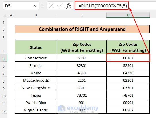
Formula Breakdown:
- The RIGHT function returns the specified number of characters from the end of a text string.
- Concatenate 00000 before each number by using Ampersand(&) between the 00000 & the cells.
- The RIGHT function allows only the last 5 characters of each resultant data to be input into the cells.
Method 5 – Use the BASE Function to Keep Leading Zeros in Excel
The BASE function is used to convert a number to different number systems (Binary, Decimal, Hexadecimal or Octal). It also allows you to choose how many characters are visible.
Steps:
- Insert the following formula in cell D5:
=BASE(C5,10,5)
- Press Enter.
- Use Fill Handle to autofill all other cells you want to populate.
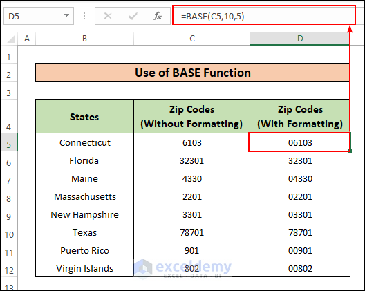
Formula Breakdown:
Inside the arguments of the BASE function,
- C5 is chosen as the cell value for C5.
- 10 is the radix or number system for decimal values.
- 5 is the number of characters we want to see as a result.
Read More: How to Keep Leading Zero in Excel Date Format
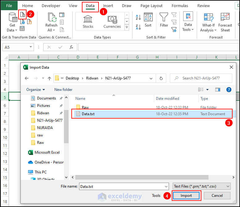
Method 6 – Import Text File & Then Use Power Query Tool & PadText Function to Add Leading Zeros in Excel
Steps:
- Under the Data ribbon, click on From Text/CSV option.
- A dialog box will appear, asking you to import the file containing the data.
- Select the file and press Import.
- Click on Transform Data in the new dialog box that appears.
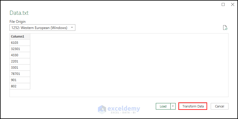
- The Power Query window will appear.
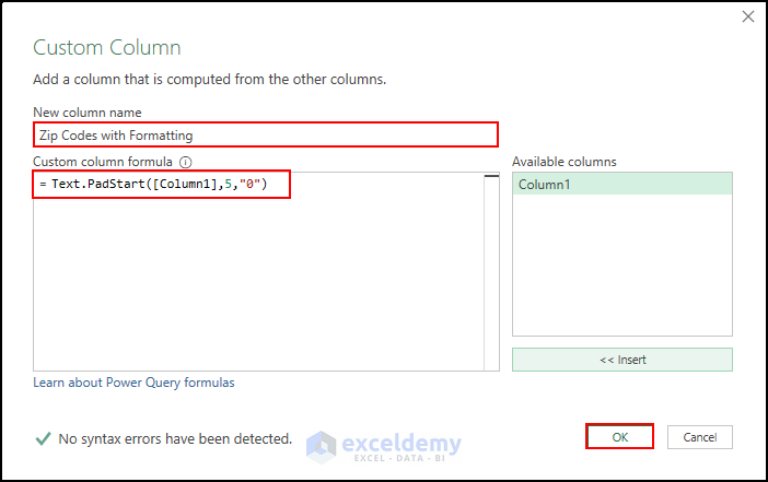
- Under the Add Column ribbon, select Custom Column.
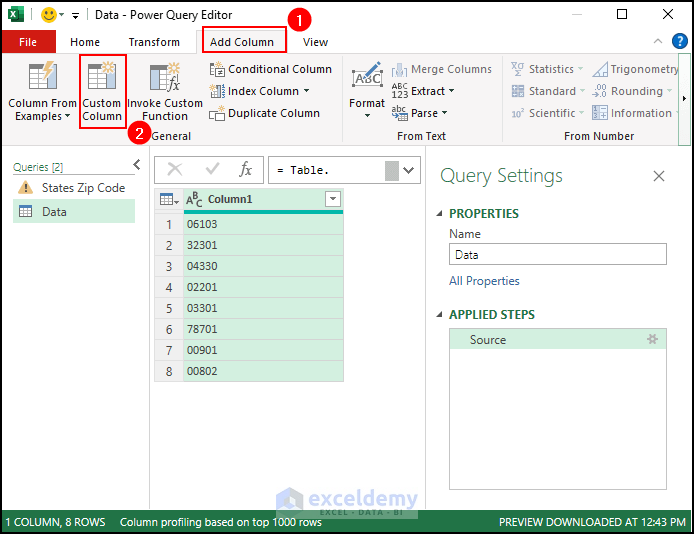
- Add the column name under the New Column Name option.
- Under the Custom Column Formula, enter:
=Text.PadStart([Column1],5,"0")
- Press OK.
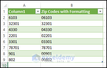
You’ll find the new column with formatted zip codes.
- Select the Close & Load option.
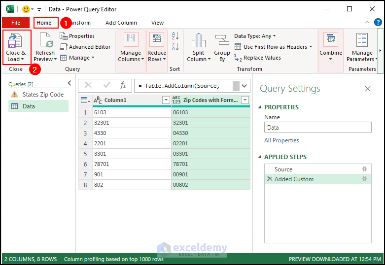
A new worksheet will appear showing the newly obtained data from the Power Query Editor as shown below.
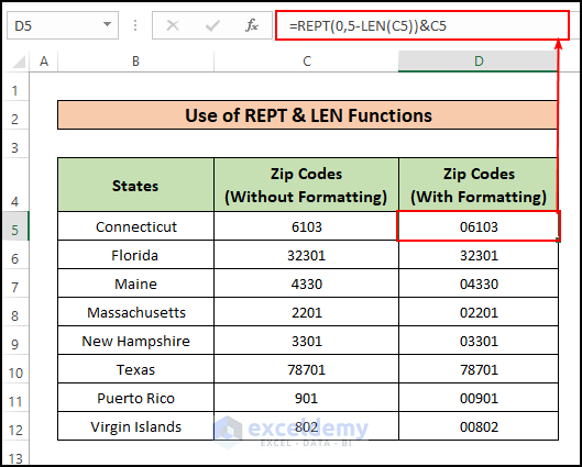
Method 7 – Merge the REPT & LEN Functions Together to Keep Leading Zeros in Excel
Steps:
- Enter the following formula in cell C5:
=REPT(0,5-LEN(C5))&C5
- Press Enter.
Formula Breakdown:
- The REPT function repeats text a given number of times.
- The LEN function returns the number of characters of a text string.
- Inside the arguments 0 has been added first as this is the text value we want to repeat as leading zeros before numbers as required.
- 5-LEN(C5) denotes the number of leading zeros that need to be added or repeated.
- Cell C5 is added to the whole function by using Ampersand(&) as this cell value has to be placed after leading zeros.
Read More: [Solved]: Leading Zero Not Showing in Excel
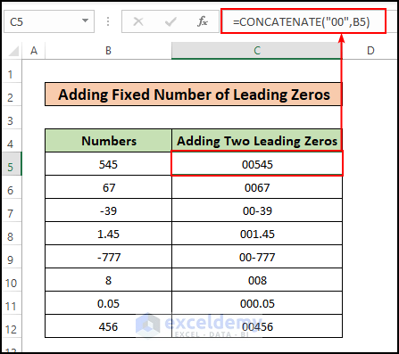
Method 8 – Use the CONCATENATE Function to Add a Fixed Number of Leading Zeros in Excel
Please note that there are different types of numbers in Column B, and here we’re going to add two leading zeros before each number.
Steps:
- Enter the following formula in cell C5:
=CONCATENATE("00",B5)
- Press Enter.
- Use the Fill Handle to autofill the other cells up to C12.
The picture below shows that each number has two leading zeros.
Method 9 – Use VBA to Keep Leading Zeros in Excel
Steps:
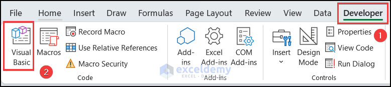
- Choose Developer in the top ribbon and then select the Visual Basic option from the menu.
- You can use ALT + F11 to open the “Microsoft Visual Basic for Applications” window if you don’t have the Developer tab added.
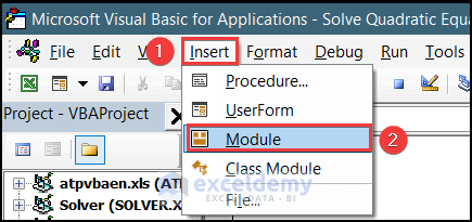
- A window named “Microsoft Visual Basic for Applications” will appear. Choose “Insert” from the top menu bar. A menu will appear. Select “Module’”.
- A new “Module” window will appear. Paste this VBA code into the box.
Sub KeepLeadingZeroes()
Range("C5", Range("C5").End(xlDown)).Select Selection.NumberFormat = "000000"
End Sub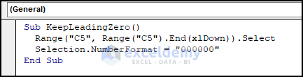
- Press F5 and the codes or macro will run.
- Press Alt+F11 again to return to your Excel spreadsheet and you’ll see the result as shown in the following picture.
VBA Code Explanation:
- The Subroutine section is added first and our macro is named KeepLeadingZeros.
- The Range command identifies the first cell that needs to be formatted.
- The End(xldown) and Select sub-commands identify the entire range of cells containing the zip codes.
- The NumberFormat sub-command defines the number of digits (5) with 0’s.
Read More: How to Remove Leading Zeros in Excel
Method 10 – Use the DAX Formula to Keep or Add Leading Zeros in a Pivot Table in Excel
Steps:
- From the Insert ribbon select Pivot Table. A dialog box named Create Pivot Table will appear.
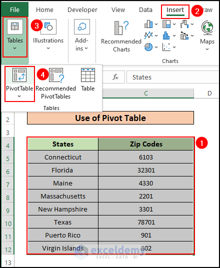
- In the Table/Range box select the whole Table Array (B4:C12).
- Mark the option ‘Add this data to the Data Model’.
- Press OK.
Your data can be converted into a pivot table where DAX measures are available.
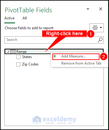
- A new worksheet will appear along with the Pivot Table Fields window on the right.
- Right-click your mouse on the Range.
- Select Add Measure.
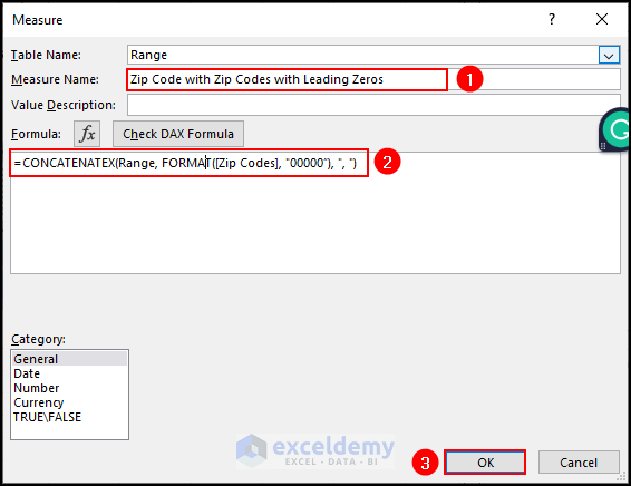
A new dialog box named Measure will appear. This is called DAX Formula Editor.
- Enter Zip Codes with Leading Zeros as Measure Name.
- Under the Formula bar, enter-
=CONCATENATEX(Range,FORMAT([Zip Codes],"00000"),",")
- Press OK.
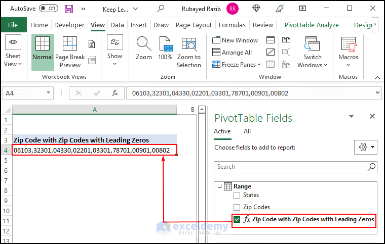
- Go to the Pivot Table Fields again and you’ll find a new option – fx Zip Codes with Leading Zeros.
- Mark this option and you’ll see the result on the left in the spreadsheet.
You can download the practice book that we’ve used to prepare this article. You can change or modify the cells & see the results at once with embedded formulas.
Related Articles
<< Go Back to Pad Zeros in Excel | Number Format | Learn Excel
Get FREE Advanced Excel Exercises with Solutions!

Unfortunately none of these methods works for me.
I have a list of article numbers. They come in lots of different ways (different lengths, only numbers, only letters, numbers+letters, some with an a – or a . or a / somewhere,… So there is no predefined special format applicable for all references.
Some are preceded by a 0 (or more 0s).
I need to use vertical lookup function to link tables.
When I copy a cell or the column, the leading 0 is still showed in the copied cell(s).
But with every action I do in excel, the leading 0 disappears. Even when I just make the cell format as “text”, the 0 still disappears. So I don’t want to add a 0, I just want to keep those that are there.
The list is also to long to add a ‘ in front of each number.
Note: When I click on a cell with a leading 0 visible in the cell, the formula bar doesn’t show that leading 0.
How to resolve?
Hi Amelie,
Thanks for your comment. As your dataset doesn’t follow any regular pattern, so I think we need an additional column to solve this issue. The procedure is:
1) First, insert a new column just right after your data column.
2) Then, at the first cell of that column, write down ‘[Value].
Here, the [Value] represents the data of the previous column.
3) Now, double-click on the Fill Handle icon.
4) The same result will be pasted on every cell. Click on the Auto Fill Options > Flash Fill option.
5) The apostrophe will add to every cell value, and it will prevent the disappearance of zero (0) from your dataset.
I hope you will be able to restore your cell values accurately. Please inform us if you are still facing any trouble.