Method 1 – Using Keyboard Shortcut
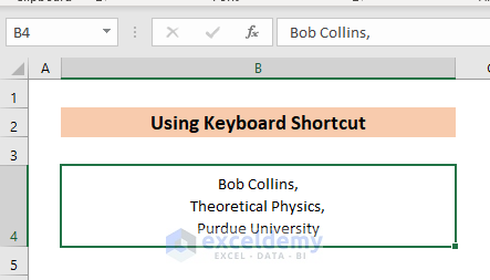
Let’s say a cell is describing a student studying a specific subject at a university. The data here is separated by commas. Let’s insert carriage returns to this cell to separate the info in three lines.
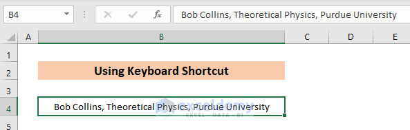
Steps:
- Take the cursor after the comma that separated the first text data.
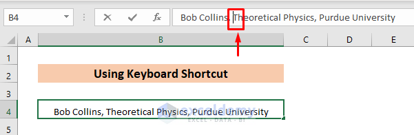
- Press Alt +Enter and you will see that a new line has been created.
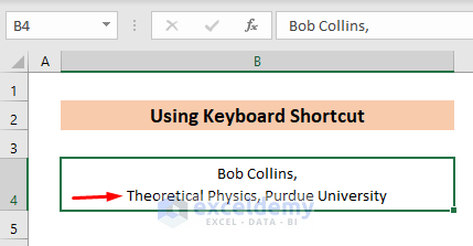
- Double-click on the cell and repeat for the next line.
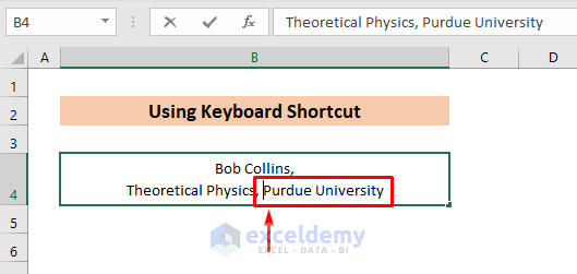
- You will find 3 new lines in a single cell for your dataset.
Read More: Remove Carriage Return in Excel with Text to Columns
Method 2 – Insert a Carriage Return Using Formula
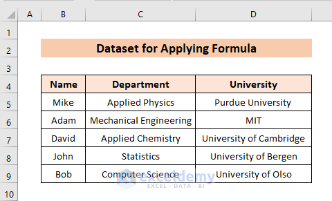
Let’s say we have a dataset of the name of some students studying in different universities and their relevant departments. We want to combine the data for each student in just a single cell and insert carriage return by applying formulas.
Case 2.1 – Applying the CHAR Function
Steps:
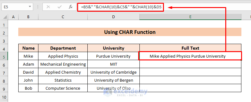
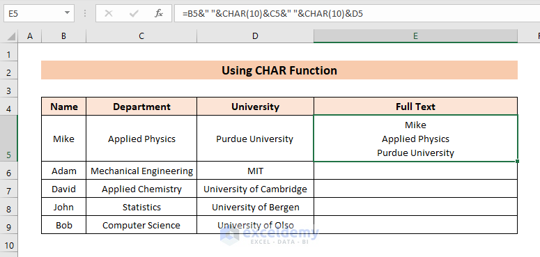
- Create a column and apply the following formula to the cell corresponding to the first student:
=B5&" "&CHAR(10)&C5&" "&CHAR(10)&D5
Here,
- B5= Name of the Student
- C5= Department
- D5= University
Formula Breakdown
- B5 & “ ”= the cell value of B5 and “ ” denotes a space after the value.
- CHAR(10)= a line break
B5&” “&CHAR(10) returns Mike.
B5&” “&CHAR(10)&C5&” “&CHAR(10) returns Mike Applied Physics.
B5&” “&CHAR(10)&C5&” “&CHAR(10)&D5 returns Mike Applied Physics Purdue University.
- Go to the Home tab and click Wrap Text.
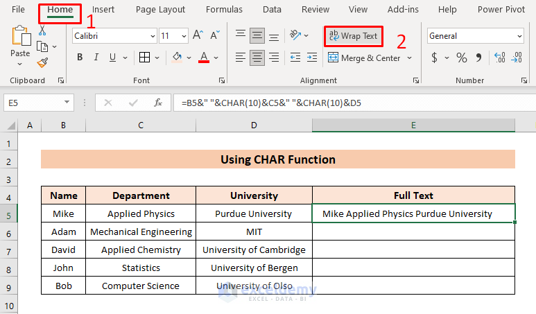
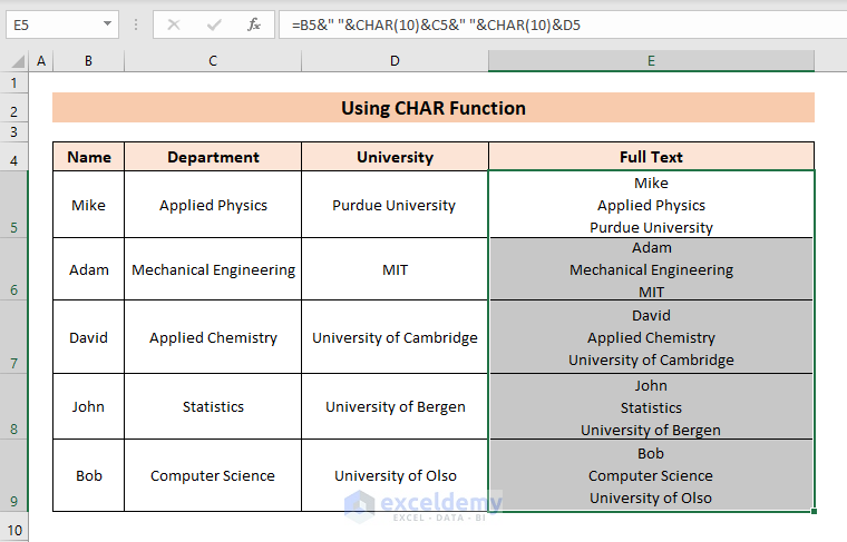
- The cell will show new lines for each piece of information (i.e. Name, Department, University).
- Use the Fill Handle tool to Autofill the formula down to the next cells.
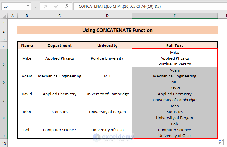
Case 2.2 – Using the CONCATENATE Function
Steps:
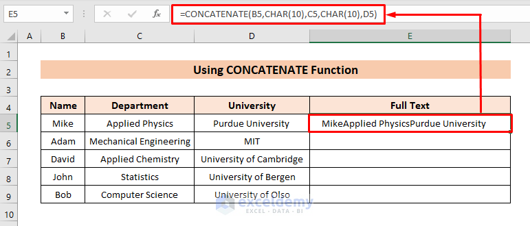
- Apply the following formula to the first result cell:
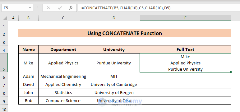
=CONCATENATE(B5,CHAR(10),C5,CHAR(10),D5)
Here,
- B5= Name of the Student
- C5= Department
- D5= University
- Use the Wrap Text option.
- Drag the formula to the other cells to get the same result.
Read More: How to Find Carriage Return in Excel
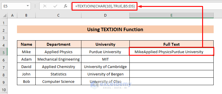
Case 2.3 – Using the TEXTJOIN Function
Steps:
- Apply the following formula to the first result cell:
=TEXTJOIN(CHAR(10),TRUE,B5:D5)
Here,
- B5= Name of the Student
- C5= Department
- D5= University
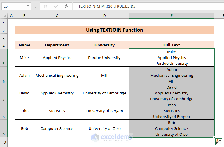
- Use Text Wrap and AutoFill to the other columns, similarly to the previous cases.
Read More: How to Replace Carriage Return with Comma in Excel
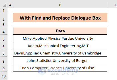
Method 3 – With the Find and Replace Dialogue Box
We have the similar dataset as in Method 1. The values are separated by commas only.
Steps:
- Press Ctrl + H to open the Find and Replace dialogue box.
- In the Find what box, input a comma.
- Select the Replace with field and press Ctrl + J.
- Click Replace All.
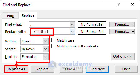
- A carriage return will be inserted instead of a comma.

Things to Remember
- Carriage return creates new lines in a single cell.
- CHAR(10) is used to insert the carriage return character.
Download Practice Workbook
You can download the practice book below.
Related Articles
<< Go Back to Carriage Return | Text Formatting | Learn Excel
Get FREE Advanced Excel Exercises with Solutions!
