How to Delete Multiple Columns in Excel with a Condition – 3 Methods

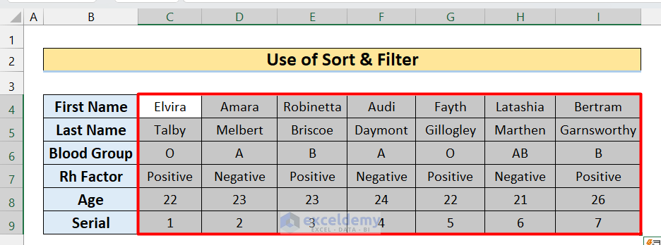
This is the sample dataset.

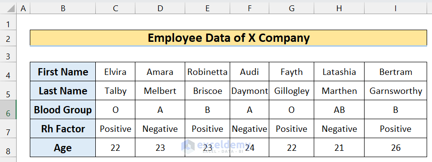
To delete multiple columns based on a condition (for example, with a negative Rh factor):

Method 1 – Use the Find & Replace Tool to Delete Multiple Columns with a Condition

Steps:

• Select the row with the condition. Here, Rh Factor.

• Press Ctrl+F to open up the Find and Replace dialog box.

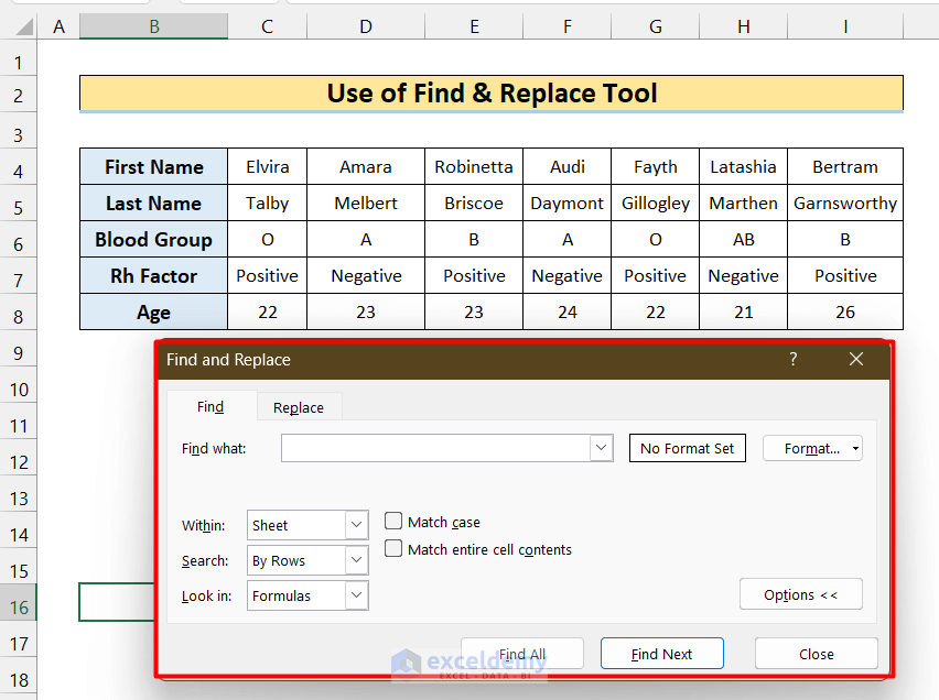
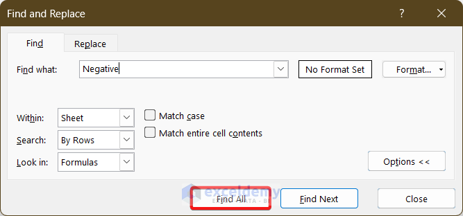
• In Find what, enter Negative and click Find All.

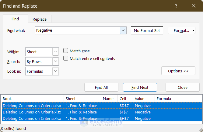
You will see the list of cells that contain this word.

• Press Ctrl+A to select those cells and close the window.

• All cells that meet the condition are selected and highlighted.
• Hold Ctrl and press the – to open the Delete dialog box.

• Select the Entire column and click OK to delete the columns that contain those cells.

Read More: How to Delete Every Other Column in Excel

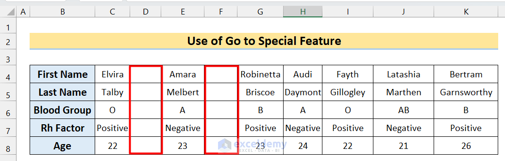
Method 2 – Deleting Multiple Columns with Blank Cells

Steps:

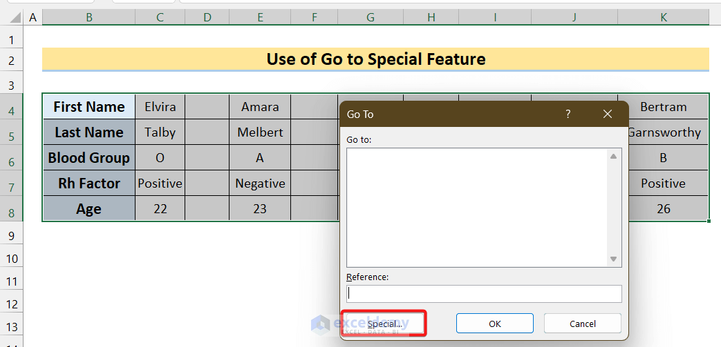
• Select the dataset and click F5 to open the Go to dialog box.
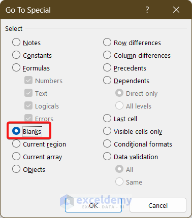
• Click Special.

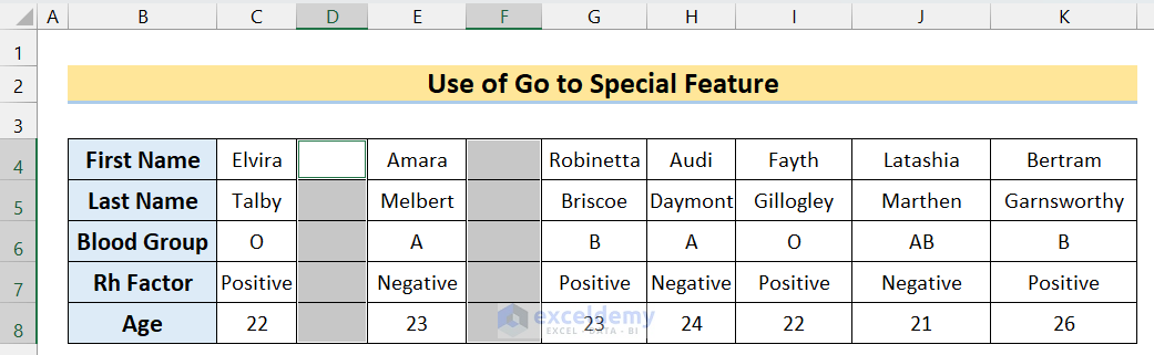
• In the Go to Special window, select Blanks and click OK.

Blank cells are highlighted.

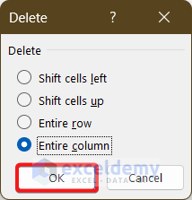
• Press Ctrl and –  to open the Delete dialog box.
• Select Entire column to see the final result.

Method 3 – Utilize the Sort & Filter Feature to Delete Multiple Columns Based on a Condition

Steps:

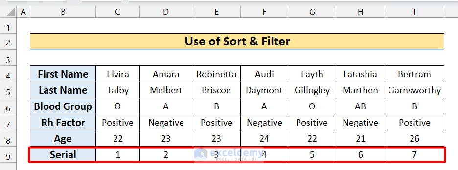
• Insert a helper row to store the serial number of the cells.

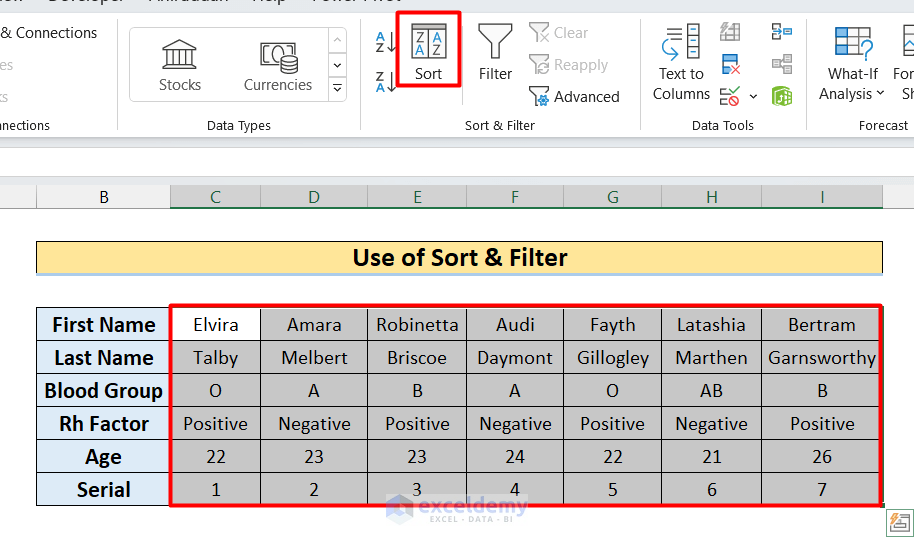
• Select the dataset (exclude the headers).

• Go to the Data tab and select Sort in Sort & Filter.

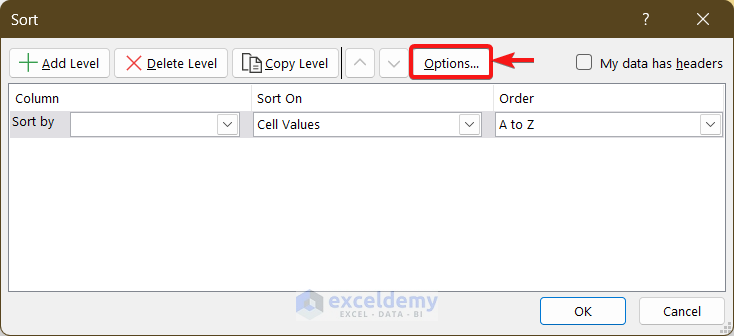
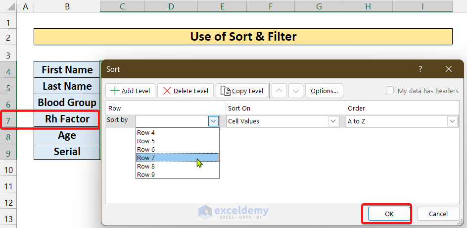
• In the Sort window, click Options.

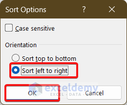
• Choose Sort left to right and click OK.

• In Sort by, select the row number based on which data will be sorted. Here, row 7 (the Rh factor).
• Click OK.

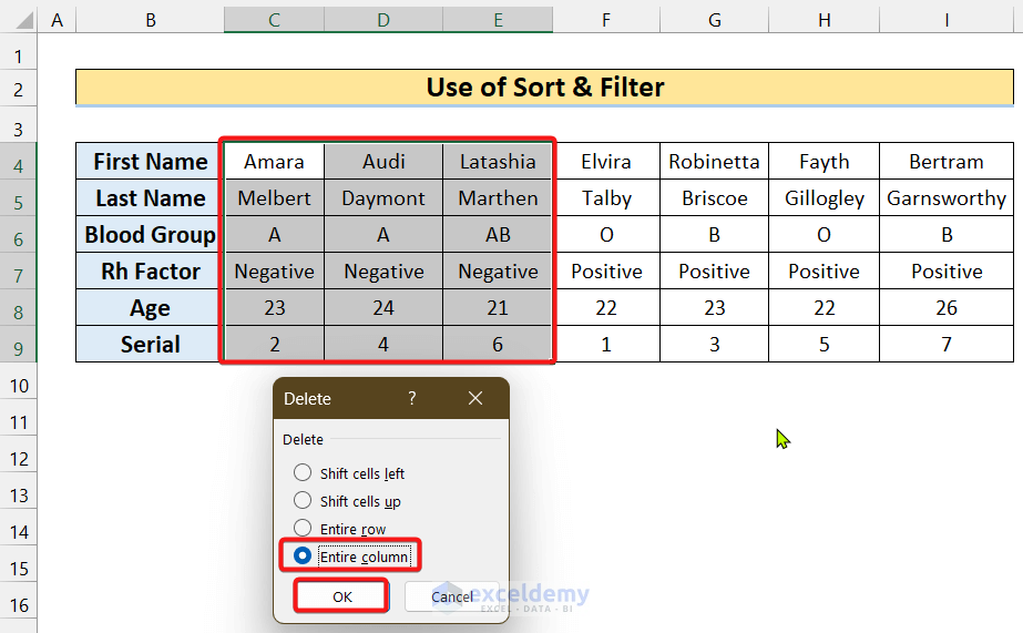
• The negative Rh factor cells are sorted. Select those cells and delete the Entire column as described in the previous methods.

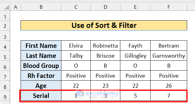
This is the output.

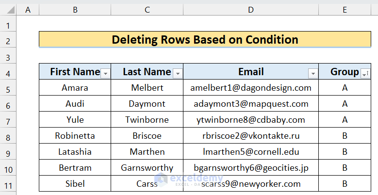
How to Delete Rows Based on Conditions

This is the dataset:

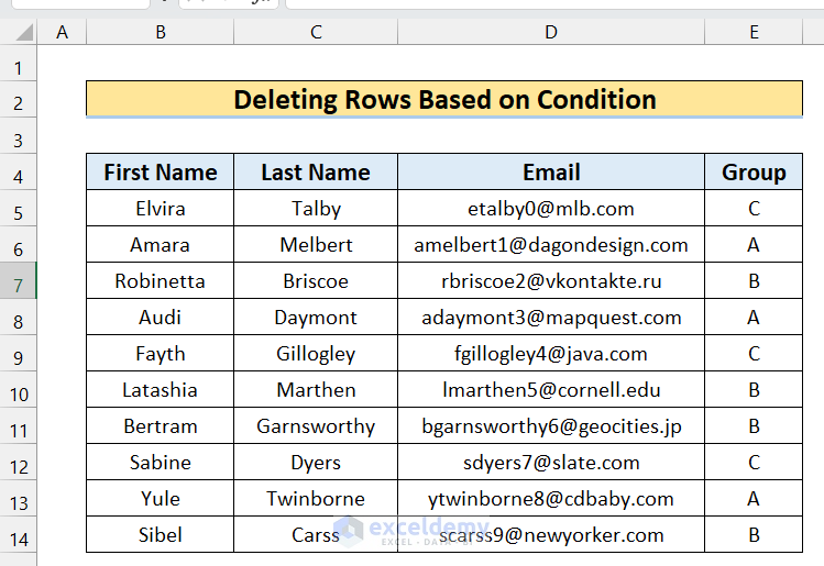
The employees are divided in 3 groups (A, B & C). To delete the rows that contain group C, use the Filter option:

Steps:

• Select the entire dataset and select Filter in the Data tab.

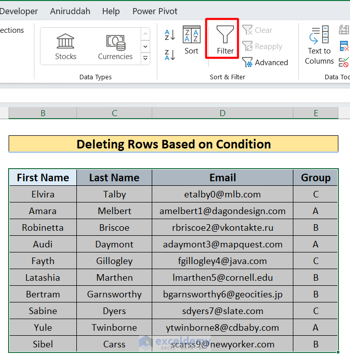
• The header column displays a filter icon.
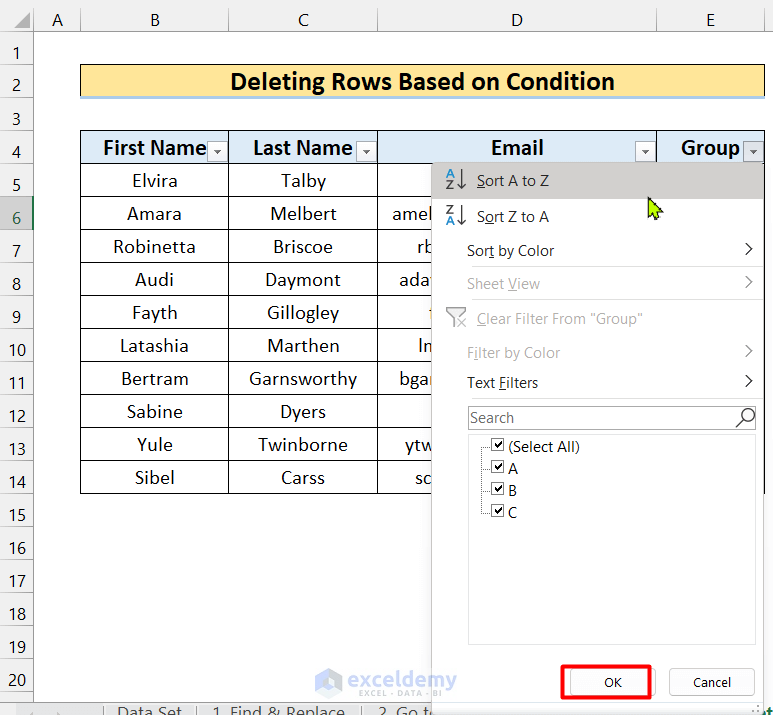
• Click the filter icon in Group and select Sort A to Z.
• Click OK.

• The list is sorted: rows containing group C are at the bottom.

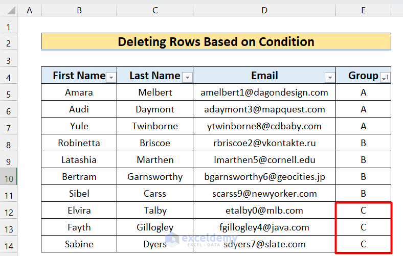
• Select those three cells and press Ctrl and – to open the Delete dialog box.

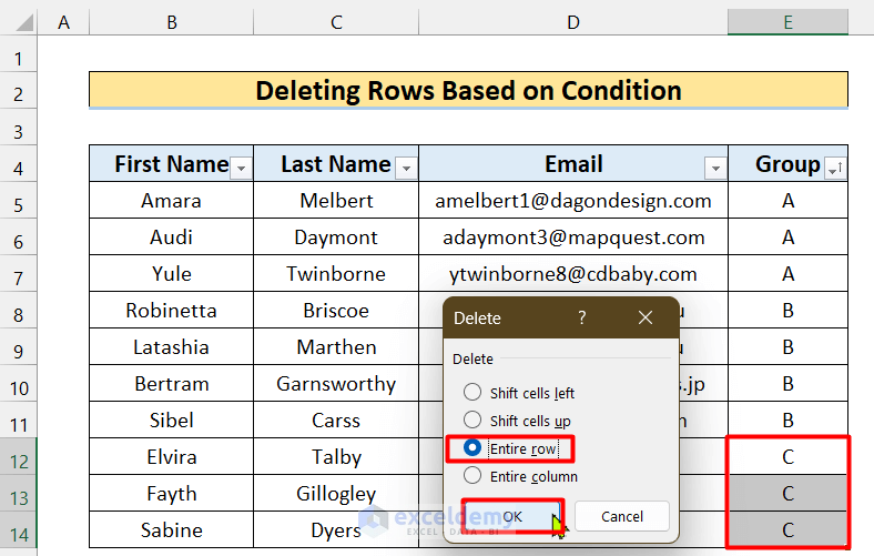
• Select the Entire row and click OK. The 3 rows will be deleted.

Download Practice Workbook

Related Articles

• How to Delete Blank Columns in Excel
• How to Delete Column in Excel Without Affecting Formula
• How to Delete Multiple Columns in Excel
• How to Delete Column in Excel Without Affecting Formula
• How to Delete Unused Columns in Excel
• How to Delete Unused Columns in Excel
• How to Delete Infinite Columns in Excel
• How to Delete Hidden Columns in Excel
• How to Delete Columns with Specific Text in Excel
• [Solved!] Can’t Delete Extra Columns in Excel

<< Go Back to Delete Columns | Learn Excel