How to Create Interactive Dashboards with Form Controls in Excel

Interactive dashboards are powerful tools for visualizing and analyzing large data dynamically in Excel. It offers a dynamic way to analyze data to get quick insights. Excel’s Form Controls are an excellent feature for creating such dashboards without VBA. It allows users to interact with data through buttons, sliders, combo boxes, and checkboxes. In this article, we will show how to create interactive dashboards with form controls in Excel.

Consider a sales dataset to show the necessary Form Controls to create an interactive dashboard.

Step 1: Prepare the Dataset

• Convert the sales data into an Excel table. Select the data range.
• Go to the Insert tab >> select Table.
  • Select My table has headers >> click OK.

• Name the table as SalesData for better readability.

Excel Table offers dynamic ranges for formulas and charts.

Step 2: Insert Form Controls and Link it to Cells

Based on your dataset type, you can select relevant Form Controls.

• Option Button (to filter by region):
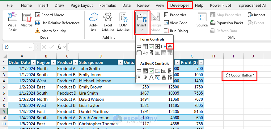
  • Go to the Developer tab >> from Insert >> select Option Button.
  • Place the Plus icon (+) on the dashboard area.
  • Right-click on the Option Button >> select Format Control.

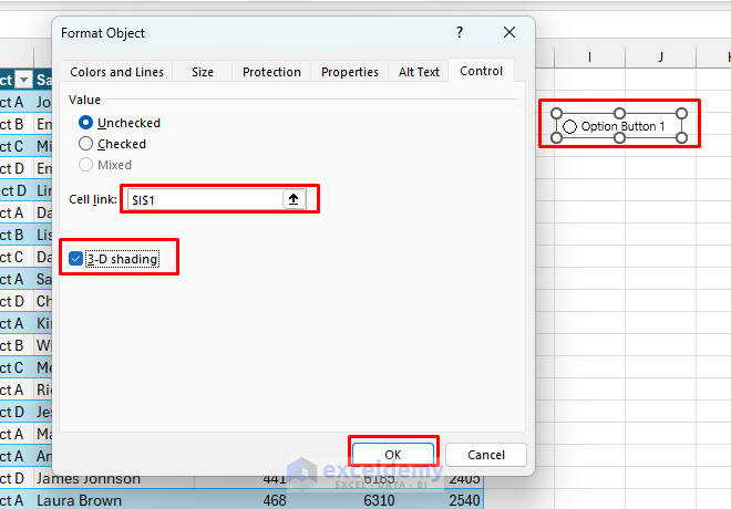
• • In the Format Object dialog box:
    • Cell link: Select cell I1 to store the selected regions.
    • Select 3-D shading >> click OK.
  • Right-click on the Option Button >> select Edit Text >> insert Regions (e.g., North, South, East, West) one by one.

• Combo Box (to filter by Product):
  • Developer Tab → Insert → Combo Box.
  • Place it on the dashboard area.
  • Go to the Developer tab >> from Insert >> select Combo Box.
  • Place the Plus icon (+) on the dashboard area.
  • Right-click on the Combo Box >> select Format Control.
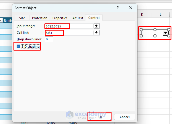
  • In the Format Object dialog box:
    • Input range:  Select the list of products (e.g., Product A, Product B, Product C, Product D).
    • Cell link: Select cell J1 to store the selected products.
    • Select 3-D shading >> click OK.

• Check Boxes (to toggle metrics like Revenue, Units Sold, and Profit):
  • Go to the Developer tab >> from Insert >> select Check Box.
  • Place the Plus icon (+) on the dashboard area.
  • Right-click on the Check Box >> select Format Control.
  • In the Format Object dialog box:
    • Cell link: Select cell K1 to store the selected metrics.
    • Select 3-D shading >> click OK.
  • Right-click on the Option Button >> select Edit Text >> insert metrics name (e.g., Revenue, Units Sold, Profit) one by one.
  • Each checkbox returns TRUE or FALSE when linked to a cell (e.g., K1, K2, K3 for Revenue, Units Sold, and Profit, respectively).

Step 3: Create Dynamic Formulas

You can use dynamic functions to link the sales data with the format controls to make the dashboard interactive. We are going to use the FILTER, SWITCH, and IF functions to extract data based on form selections dynamically.

Using Dynamic FILTER Function

Filter Data by Region:

Insert the following formula in the selected cell to filter sales data based on selected regions.

=FILTER(SalesData, SalesData[Region] = SWITCH(J1, 1, "North", 2, "South", 3, "East", 4, "West"))

• Filter function extracts the SalesData table to display the rows where the Region matches the selected value in cell J1.
• The SWITCH function translates the numeric value in J1 (e.g., 1, 2, 3, or 4) into corresponding region names (“North,” “South,” “East,” or “West”). Only matching rows are included in the result.

Filter Data by Product:

Insert the following formula in the selected cell to filter sales data based on selected products.

=FILTER(SalesData, SalesData[Product] = SWITCH(K1, 1, "Product A", 2, "Product B", 3, "Product C", 4, "Product D"))

This formula will filter the sales data based on the selection of combo boxes. We selected Product A from the combo box so it will return Product A’s sales data.

Filter Data by Region & Product:

Insert the following formula in the selected cell to filter sales data based on selected regions and products.

=FILTER(SalesData, (SalesData[Region] = SWITCH(J1, 1, "North", 2, "South", 3, "East", 4, "West")) * (SalesData[Product] = SWITCH(K1, 1, "Product A", 2, "Product B", 3, "Product C", 4, "Product D")))

This formula will filter the sales data based on the selection of a combo box and option button. We selected the South region and Product B. Filter function will return only the sales information of Product B from the South region.

Dynamic Metric Display

You can use the IF function to display the sales metrics based on the check box selection.

Insert the following conditional logic for metrics based on the checkbox values. If you select any checkbox it returns TRUE otherwise FALSE in the linked cell. Based on the value of the linked cell the IF function will return the result.

Revenue:

Insert the following formula to get the total revenue.

=IF(L1, SUM(SalesData4[Revenue ($)]), "")

To get the totals from the filtered sales data, insert the following formula:

=IF(L1, SUM(O9:O30), "")

These formulas will sum the revenue if you select the checkbox of Revenue.

Profit:

Insert the following formula to get the total profit.

=IF(M1, SUM(SalesData4[Profit ($)]), "")

To get the totals from the filtered sales data, insert the following formula:

=IF(M1, SUM(P9:P30), "")

These formulas will sum the profit if you select the checkbox of Profit.

Units Sold:

Insert the following formula to get the total units sold.

=IF(N1, SUM(SalesData4[Units Sold]), "")

To get the totals from the filtered sales data, insert the following formula:

=IF(N1, SUM(N9:N30), "")

These formulas will sum the total units if you select the checkbox of Units Sold.

Output:

Step 4: Insert Dynamic Charts

• Select the filtered data.
• Go to the Insert tab >> click on All Charts >> select Column chart.

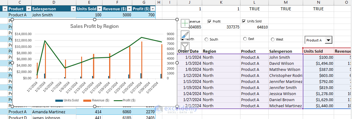
• The charts will update automatically based on the Combo Box and Option Button. This chart showing the sales of the Product A in the North region.

• Change the filter option to see the dynamic update of the chart. We selected East region and Product C.

Step 5: Customize the Dashboard

• Insert Shapes:
  • Add different as per your dashboard requirements to separate sections like filters, charts, and metrics.
• Formatting:
  • You can use consistent colors, fonts, and styles.
  • You can use conditional formatting to highlight.

Conclusion

With the above steps, you can create interactive dashboards with form controls in Excel. We have shown all the important steps by creating an interactive, visually appealing dashboard using a large dataset. You can dynamically filter and analyze data, making it a powerful tool for decision-making. Do not forget to experiment with additional features of form controls.