How to Build Real-Time Data Dashboards with Power Query

Excel’s Power Query is one of the most powerful tools for data connection, transformation, and real-time updates. Power Query can import data from various sources and refresh it in real time whenever there are changes in the source data. In this article, we will show how to build real-time data dashboards with Power Query.

Let’s create a real-time sales dashboard by performing additional operations in Power Query on the expanded dataset. The headers in the sales dataset include Order Date, Region, Product, Salesperson, Units Sold, Revenue ($), and Profit ($).

Step 1: Connect Data with Power Query

To get data from external sources:

• Go to the Data tab >> select Get Data >> From File >> From Workbook.
• Select your dataset file (e.g., SalesData.xlsx) and click Import.
• In the Navigator, select the sheet with the sales data and click Load.

To connect data from the existing workbook:

• Go to the Data tab >> select From Table/Range.

Power Query will load the data into the Power Query Editor.

Step 2: Transform the Data with Advanced Operations

Now the data is loaded into the Power Query Editor, let’s perform data transformations and calculations.

1. Change Column Data Types

Power Query sometimes changes data formats to its default format. Based on your data type, change the whole column.

• Order Date: Make sure it’s in Date format.
  • If not, select the Date column.
  • Go to the Transform tab >> from DataType >> select only Date.
• Units Sold: Check if it is in Whole Number format.
  • If not, select the Units Sold column.
  • Go to the Transform tab >> from DataType >> select only Whole Number.
• Revenue ($) and Profit ($): Ensure these columns are in Currency format.
  • If not, select the Revenue ($) and Profit ($) columns.
  • Go to the Transform tab >> from DataType >> select only Currency.

2. Add a “Month” Column

• Select the Order Date column.
• Go to the Add Column tab >> click Date >> select Month >> select Name of Month.
• This will create a column that extracts the name of the month from the Order Date (e.g., January, February).

3. Calculate Revenue per Unit

Let’s calculate the revenue generated for each unit sold.

• Go to the Add Column tab >> select Custom Column.
• In the Custom Column dialog box;
  • Name the column Revenue per Unit and use the following formula in the formula box:

[#"Revenue ($)"]/[Units Sold]

• • Click OK.

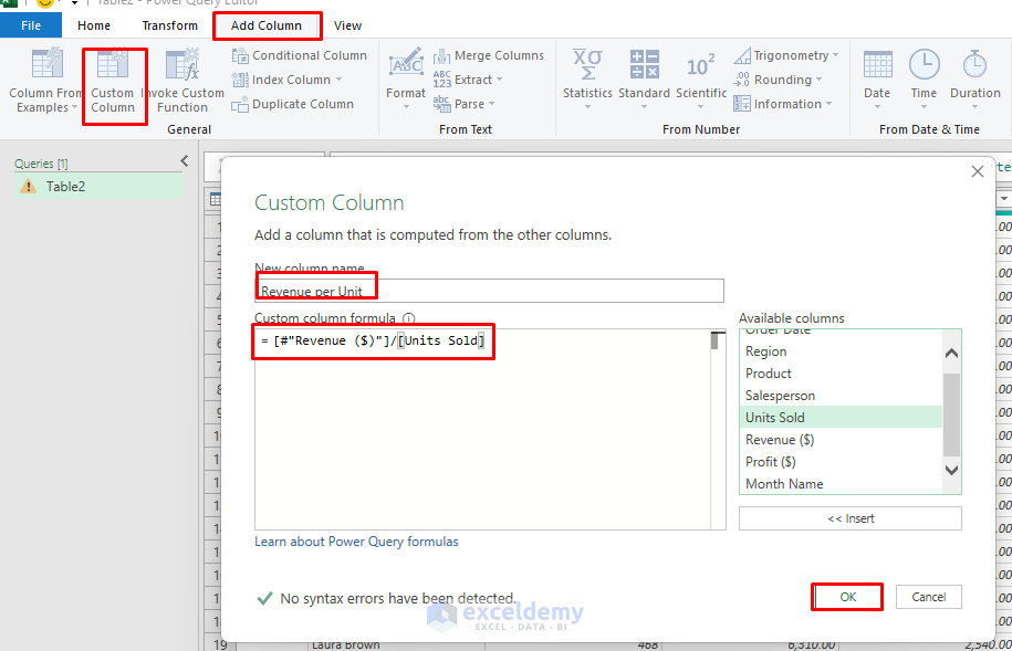
This new custom column will show how much revenue was generated for each unit sold.

4. Calculate Profit Margin

Next, let’s calculate the Profit Margin. The profit margin is calculated as:

• Go to the Add Column tab >> select Custom Column.
• In the Custom Column dialog box;
  • Name the column Profit Margin (%) and use the following formula in the formula box:

([#"Profit ($)"]/[#"Revenue ($)"])*100)

• • Click OK.

This custom column will show the profit margin for each sale.

5. Group Data by Region and Product for Aggregated Insights

To see the total Revenue, Units Sold, and Profit by Region and Product, we’ll group the data.

• Go to the Home tab >> select Group By.
• In the Group By dialog box, set the following:
  • Select Advanced to add multiple aggregations.
  • Group by: Region, Product.
  • Insert Valid New columns name.
  • Operation: Sum 
  • Column:
    • Units Sold
    • Revenue ($)
    • Profit ($)
  • Click OK.

The Group By feature will summarize the data by Region and Product, to provide an overview of sales performance.

6. Sort the Data

Sort the data by Revenue ($) in descending order to view the top-performing products and regions.

• Click the dropdown on the Revenue ($) column header.
• Select Sort Descending >> click OK.

This will sort your data to show the data from highest to lowest based on Revenue.

Step 3: Load the Transformed Data into Excel

To load the cleaned and transformed data into an Excel worksheet.

• Go to the Home tab >> from Close & Load >> select Close & Load.

Step 4: Creating a Dashboard

When your data is transformed and loaded into Excel, you can create a dashboard with visualizations.

1. Create a Pivot Table

• Choose the transformed data table.
• Go to Insert tab >> select PivotTable.

• In the PivotTable Fields List:
  • Rows: Region, Product.
  • Values: Sum of Units Sold, Sum of Revenue, Sum of Profit.

2. Create Pivot Charts

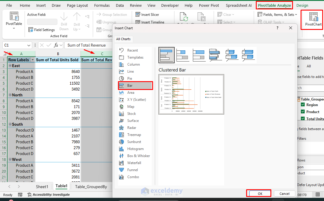
Bar Chart for Revenue by Region:

• Highlight the Pivot Table with Region and Revenue.
• Go to PivotTable Analyze tab >> select Bar Chart >> select Clustered Bar.

Pie Chart for Sales Distribution by Product:

• Select the Pivot Table with Product and Revenue.
• Go to PivotTable Analyze tab >> select Pie Chart.

Let’s explore the interactivity of the dashboard. Select region East from the Pie chart.

You can add Slicers for Salesperson and Timeline for Order Date for Interactivity.

Step 5: Set Up Real-Time Refresh

To update the real-time data in dashboards:

• Go to the Data tab >> click Refresh All whenever you add new data to your source data.

Or you can set the workbook to refresh automatically every few minutes:

• Go to the Data tab >> select Queries and Connections >> right-click on Queries and Connections >> select Properties.

• In the Query Properties dialog box;
  • Enable Refresh every 5 minutes.
  • Click OK.

Conclusion

By following these steps, you can build a dynamic, real-time sales data dashboard using Power Query. You can perform advanced operations in the Power Query editor, to group, calculate custom columns, sort, filter, etc, and then load the transformed data into Excel to build a real-time dashboard. Power Query’s data connections and transformation feature will quickly update your dashboard with fresh data in real time.