Are you looking for an easy way to create GST late fees calculator in Excel? Don’t worry! You have landed in the right place. In this article, I will show you how to create GST late fees calculator in Excel.
What Is GST?
GST stands for Goods and Service Tax. This is a value-added tax imposed on goods and services for domestic purposes. The final price of a good or service includes this tax. Although the consumer pays this tax, it is remitted to the government by the seller or the business.
How to Create GST Late Fees Calculator in Excel: with Easy Steps
In this section, you will find some easy steps to create a GST late fees calculator in Excel. I will demonstrate them here with proper illustrations.
Just proceed with the following steps.
Step 1: Create Variable for GST Calculator
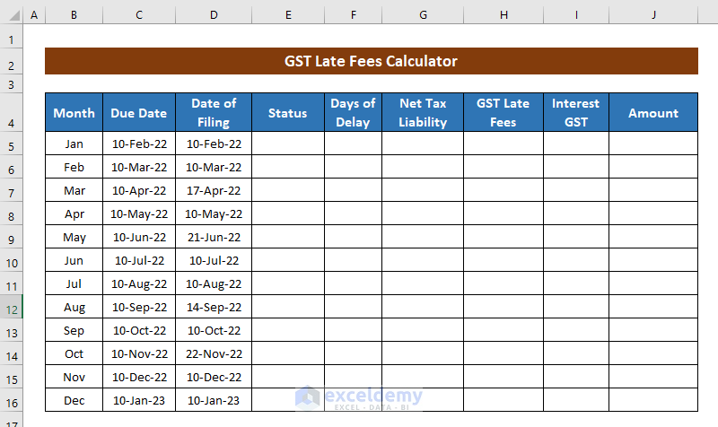
- First of all, assign variable names for calculating GST late fees and put them in the column headings. I have assigned the following variable names for my calculator:
- Month
- Due Date
- Date of Filling
- Status
- Days of Delay
- Net Tax Liability
- GST/Day if Taxable
- Interest GST
- Amount
You can add or remove any variable name as per your need.

- Then, assign the Month and Due Date to file GST. I have created my calculator for the whole year( from January to December) and taken the Due Date 10th for every month.

Step 2: GST Filing Status for Calculator
- Now, put the Date of Filing GST for every month.
- After putting the filing date in the respective column, you have to find out whether GST is filed on time or delayed. For getting the filing status we will now use the IF Function. Select the first cell of the Status column and type the following formula:
=IF(D5<=C5,"On Time","Delayed")
Here,
- D5 = Date of Filing
- C5 = Due Date
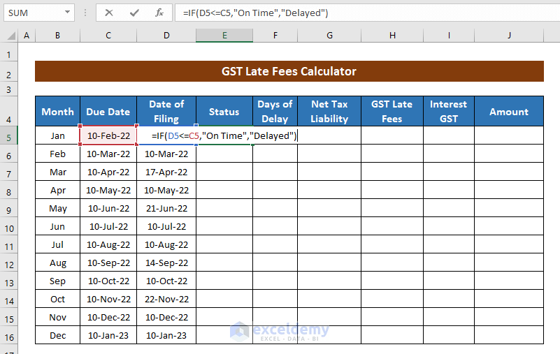
- Now, press ENTER, and the cell will show the GST filing status (On Time/ Delayed).
- Here, use the Fill Handle tool to AutoFill the formula for the rest of the cells.
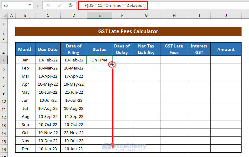
- Hence, you will get the status for all corresponding months.

- After that, find out the Days of Delay. Apply the following formula to the column Days of Delay for this:
=D5-C5
Here,
- D5 = Date of Filing
- C5 = Due Date

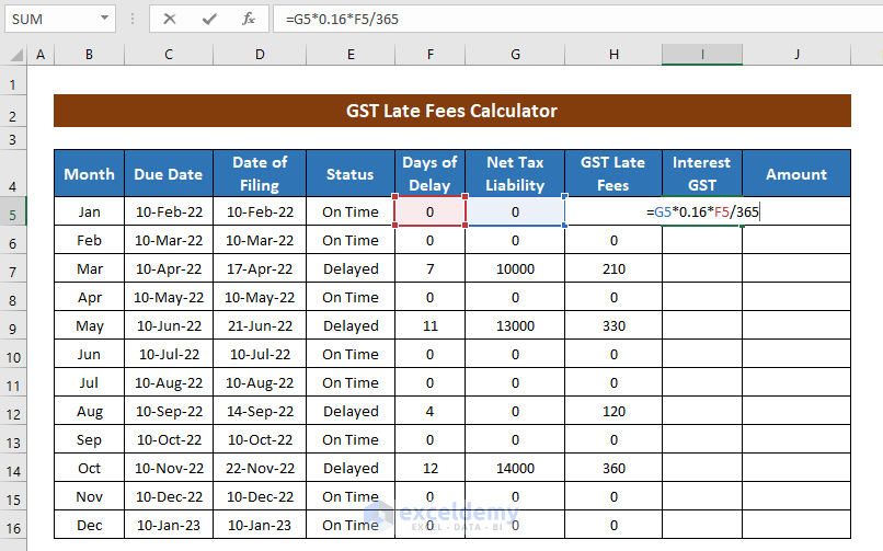
- Here, in our calculator, we have found the GST status has been Delayed four times.

Step 3: Calculate GST Late Fees
Hang on! It’s time to calculate GST Late Fees. Let’s move on.
- Assign Net Tax Liability for the concerning months. In our dataset, we have Net Tax Liability 3 times. For your case, find it from your notice and assign them as per the direction.

- Now, calculate the GST Late Fees for the number of Delayed Days. We have considered Late Fees Per Day: 30.
So to get the total late fees, multiply the number of Delayed Days with Late Fees Per Day. In order to get the total late fees, select a cell and apply the following formula:
=F5*30
Here,
- F5 = Days of delay
- 30 = Late fees per day

- Now, hit ENTER and drag the formula down for the other cells and you will get the GST Late Fees for the whole year.

Step 4: Calculate Interest on GST
Interest will be counted for the months you haven’t paid the GST on time. We have considered the Interest Rate as 16%. You can proceed with your own.
- Here, select the first cell of the Interest GST column and apply the following formula.
=G5*0.16*F5/365
Here,
- G5 = GST late fees
- F5 = Days of Delay
💡 Formula Breakdown
G5*0.16/365 gives the interest rest per day on a year. Multiplying it by F5 (Days of Delay) returns the interest over the total days of delay.
- Now, hit ENTER and drag the formula for the other cells.

Step 5: Calculate Total Payable Amount
- In order to calculate the total amounts to be paid for every month, apply the following formula:
=H5+I5
Here,
- H5 = GST late fees
- I5 = Interest on GST
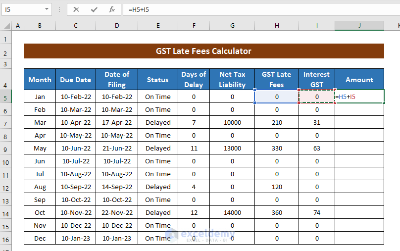
- Press ENTER and drag the formula for each cell up to the month of December.

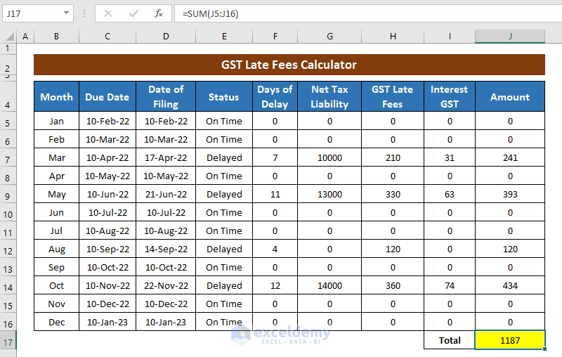
- Now, apply the following formula to get the total amount to be paid for the whole concerning time (i.e. from January to December).
=SUM(J5:J16)
Here,
(J5:J16) = the range to sum

- Finally, press ENTER to get the total amount.
Download Practice Workbook
You can download the practice book from the link below.
Conclusion
In this article, I have tried to show you the process of creating a GST late fees calculator in Excel. Hope you like reading this. If you have better methods, questions, or feedback regarding this article, please don’t forget to share them in the comment box.
Happy Excel!
Related Articles
- Computation of Income Tax Format in Excel for Companies
- Self Employment Tax Calculator in Excel Spreadsheet
- Income Tax Computation in Excel Format
<< Go Back to Excel Tax Calculator | Finance Templates | Excel Templates
Get FREE Advanced Excel Exercises with Solutions!
