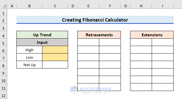
Method 1 – Insert Format of Fibonacci Calculator
- Insert a format of the calculator.
- We have our format for the Up Trend.
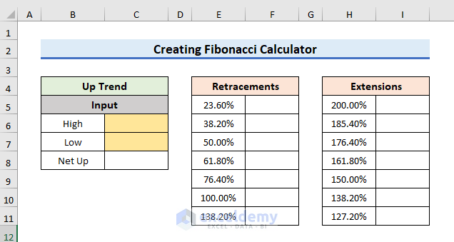
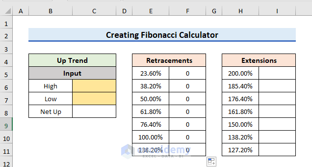
Method 2 – Add Retracements and Extensions in the Calculator
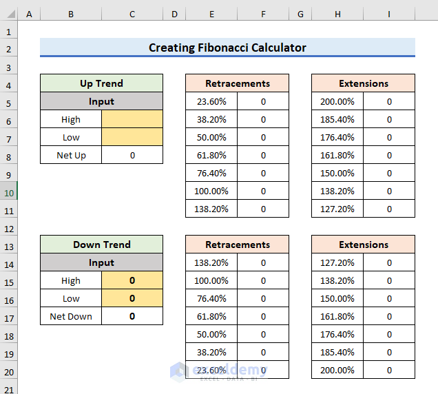
- Add Retracements and Extensions in the format of the calculator.
- The common Fibonacci ratios are 23.6%, 38.2%, 50%, 61.8%, 78.6%, 100%, and 123.20%.
- Add Retracements accordingly.
- Add Extensions to the calculator.
Method 3 – Link Between Cells to Create Calculator
- Link between input and output in the calculator.
- Link between Retracement and Extension cells and input cells.
- High and Low are our input.
- Write the following formula in the F5 cell:
=$C$6-$C$8*E5
- Press Enter to exit from the editing mode.
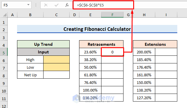
Here, $C$6-$C$8*E5 indicates that we will use the formula for a specific Retracement that is High Value – Net Up*Retracement.
- Drag down the formula in the Retracements column using the following (+) icon.
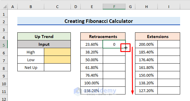
- The formula is applied to the column.
- The column is showing the value 0 as we have not inserted the input value yet.
- Write the following formula in the I5 cell:
=$C$6+$C$8*H5
- Press Enter to exit from the editing mode.
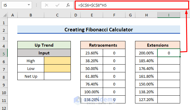
Here, $C$6+$C$8*H5 indicates that we will use the formula for a specific Extension that is High value + Net Up*Extension.
- Drag down the formula in the Extensions column using the Fill Handle.
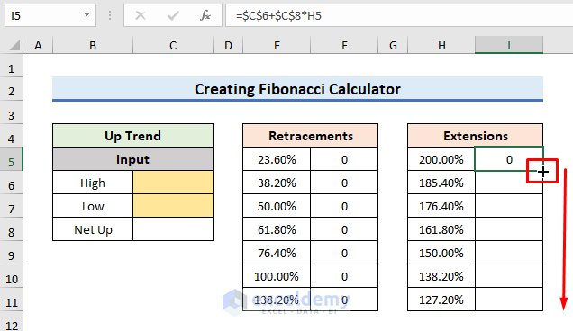
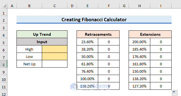
- The formula is now inserted into the Extensions column.
- The result is showing 0 as we have not inserted the value in the input.
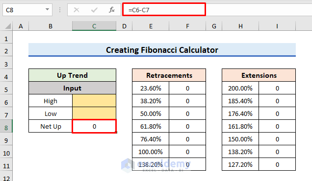
- You need the value of Net Up.
- You need to calculate the value of Net Up.
- Write the following formula in the C8 cell:
=C6-C7
- Click Enter to proceed.
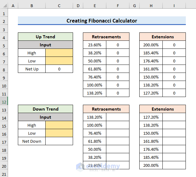
Method 4 – Insert Format for Down Trend
- For the Down Trend, we will add Retracements and Extensions.
- Write down the formula to calculate Retracements for the Down Trend.
- Write down the following formula in the F14 cell:
=$C$16+$C$17*E14
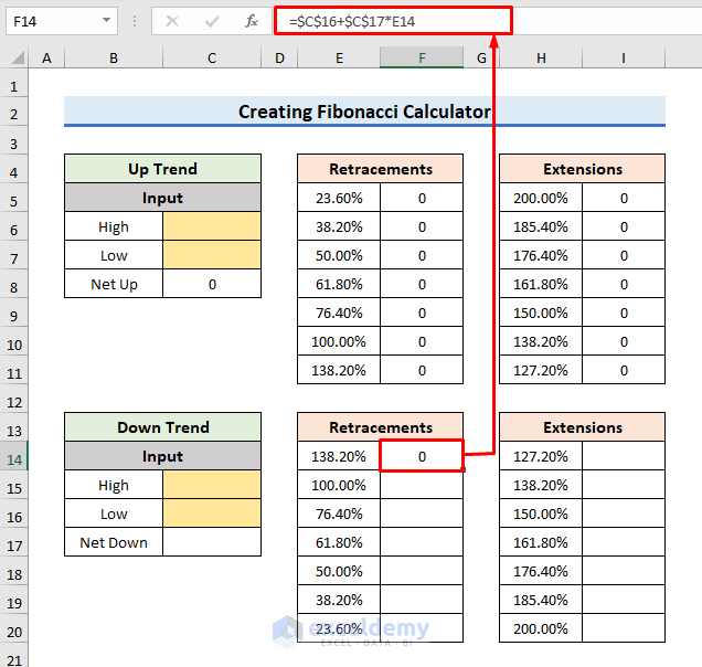
Here, $C$16+$C$17*E14 indicates that we are using the formula for a specific Down Trend’s Retracement which is Low Value + Net Down*Retracement.
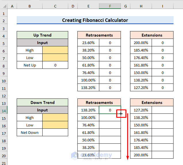
- Drag down the formula in the Retracements column using the Fill Handle.
- Write down the formula to calculate Extensions for the Down Trend.
- Write down the following formula in the I14 cell:
=$C$16-$C$17*H14
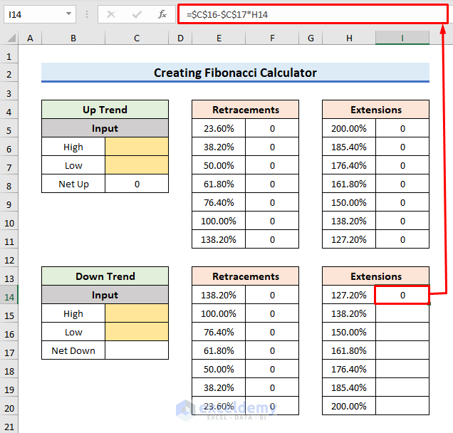
Here, $C$16-$C$17*H14 indicates that we are using the formula for a specific Down Trend’s Extension that is Low Value – Net Down*Extension.
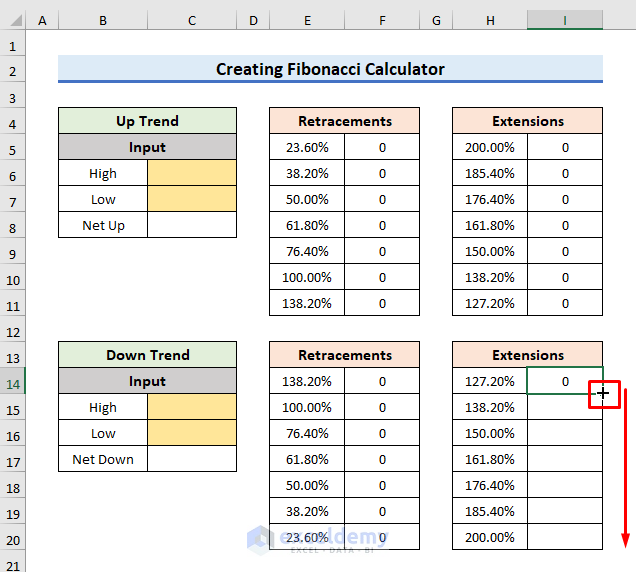
- Drag down the formula in the Extensions column using the Fill Handle.
- You don’t want to insert the input 2 times.
- Insert the input for a single time and show the output for Up and Down Trend’s Retracements and Extensions.
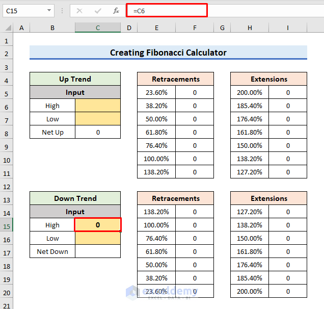
- Create a link between the inputs of Up Trend and Down Trend.
- In the C15 cell, insert the following formula in the formula bar:
=C6
- Press Enter to exit from the editing mode.
- The insert in the C6 cell is the input will show in the C15 cell.
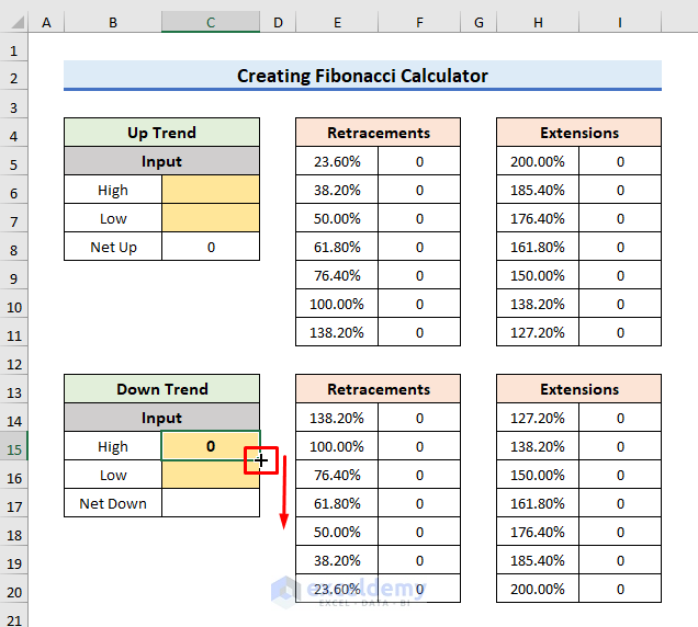
- Drag down the formula using the Fill Handle to link the Low and Net values.
Method 5 – Final Output
- The Fibonacci Calculator is ready.
- Insert the input in the C6 and C7 cells.
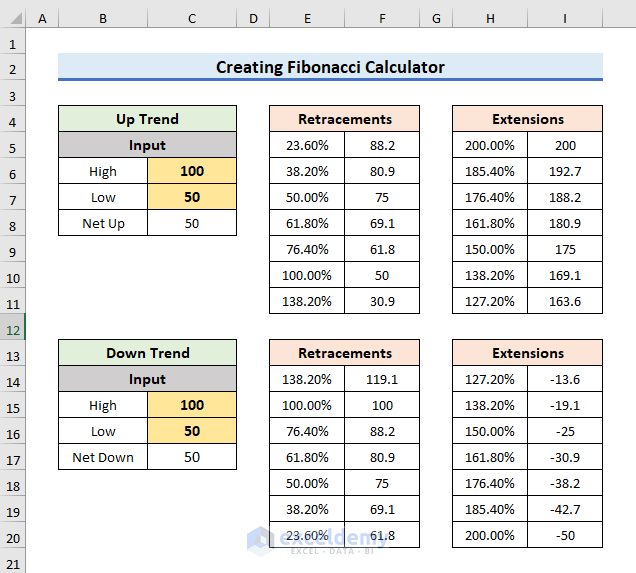
- Inserting the High value in C6 and the Low value in C7 will show the result.
- Insert the High value as 100 and the Low value as 50.
- Retracements and Extensions for Up and Down Trends are showing.
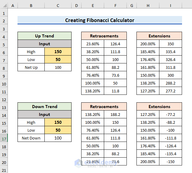
- Check for another value.
- Insert the High value as 100 and the Low value as 50.
- Retracements and Extensions for Up and Down Trends are showing.
How to Generate Fibonacci Sequence in Excel
Method 6 – Insert Initial Sequence of Fibonacci Number
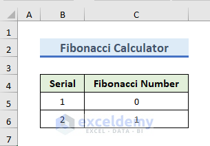
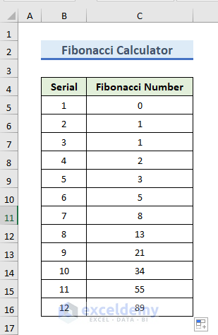
- Ggive input the first 2 numbers of the Fibonacci sequence.
- The first 2 numbers of the Fibonacci sequence are 0 and 1.
- In cell C5, insert the number 0.
- This indicates that 1st number of the Fibonacci series is 0.
- In the C6 cell, give the input as 1.
- It indicates that the 2nd number of the Fibonacci series is 1.
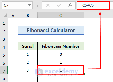
Method 7 – Apply Formula to Calculate Next Sequence
- We will calculate the 3rd number of the sequence.
- Insert the following formula in the formula bar of the C7 cell.
=C5+C6- We can see the 3rd serial of the Fibonacci sequence.
- Instead of inserting the serial number manually, we can also generate the Serial column in Excel.
- Write down the following formula in the B8 cell to sequentially increase the Serial column:
=B7+1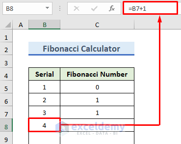
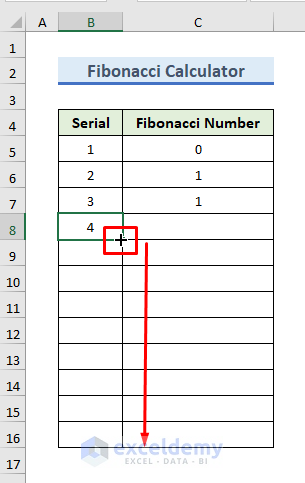
- Dag down the formula in the Serial column using the following (+) icon to generate the serial number.
- Drag down the formula of the Fibonacci sequence in the Fibonacci Number column.
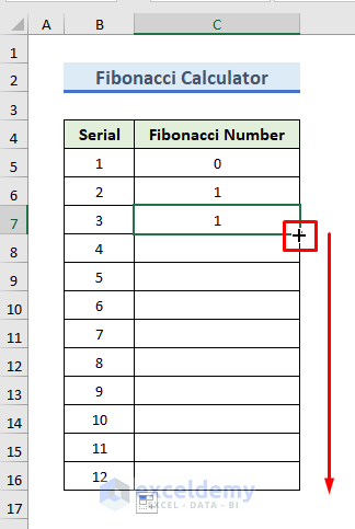
Method 8 – Final Output
- With the drag down option, you can extend the sequence as per your requirements.
Download Practice Workbook
To practice by yourself, download the following workbook.
Related Articles
- Dividend Reinvestment Calculator with Monthly Contributions in Excel
- How to Create Mortgage Loan Pipeline Management in Excel
- How to Create a Fibonacci Pivot Point Calculator in Excel
<< Go Back to Finance Template | Excel Templates
Get FREE Advanced Excel Exercises with Solutions!
