What Is Extrapolation?
Extrapolation is the prediction or estimation of unknown data based on known data assuming that the current trend continues. The mathematical equation for linear extrapolation is given below.
y(x) = y1 + [(x - x1) / (x2 - x1)] * (y2 - y1)
We have a dataset given below in the B4:D6 cells where the Month’s Name and the Month number are shown along with the Sales amount.
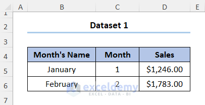
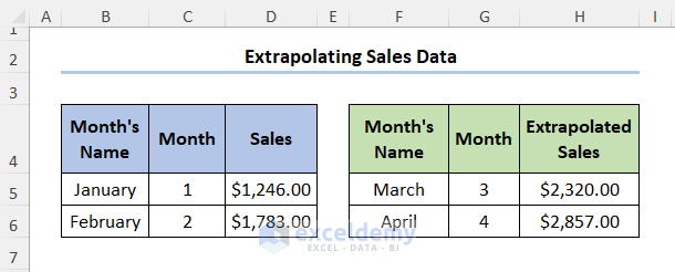
Let’s say we have the data for January and February and assume that we’ll have linear growth for the following months. We can predict the Sales for March using the extrapolation formula as shown below:
=D5+(G5-C5)/(C6-C5)*(D6-D5)
D5 and D6 cells refer to the Sales amount of $1,246 and $1,783, respectively, whereas the C5 and C6 cells indicate the Month numbers 1 and 2. G5 contains the March month number, or the new x value where the formula is calculating the y.

Copying the formula to the next cell obtains the results for April.
How to Extrapolate a Trendline in Excel: 4 Methods
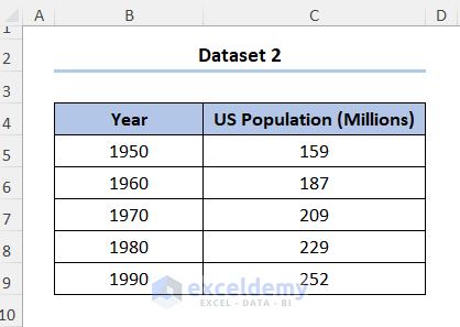
We’ll use the dataset in the B4:C9 cells, which contains the U.S. Population data for each decade starting from the 1950.
Method 1 – Extrapolating a Linear Trendline in Chart
Step 1 – Insert a Line Chart
- Insert 3 new rows in the Year column.
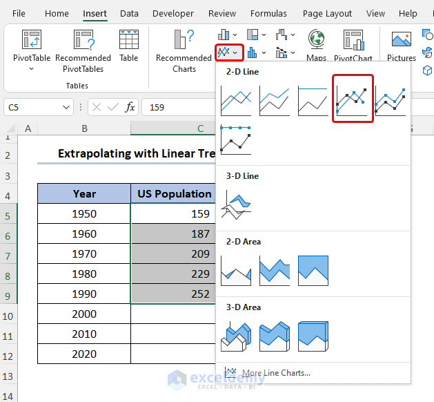
- Navigate to the Insert tab and select the Line Chart drop-down.
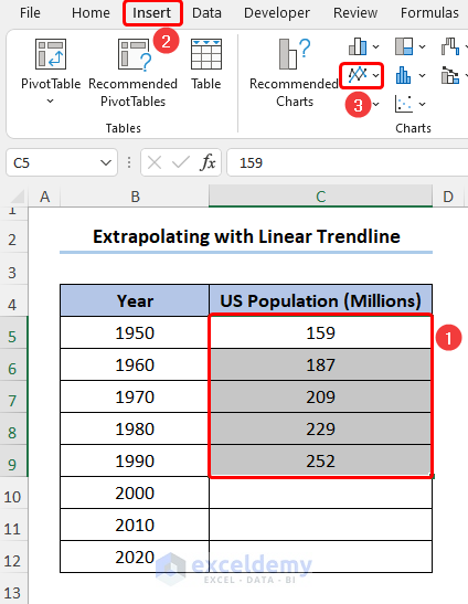
- Choose the 2D Line Chart as shown in the image below.
Step 2 – Enter Chart Data
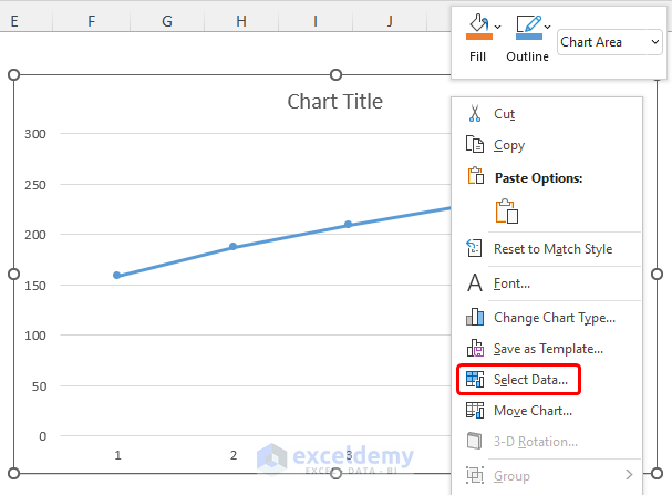
- Go to the chart and right-click on it.
- Choose the Select Data option.
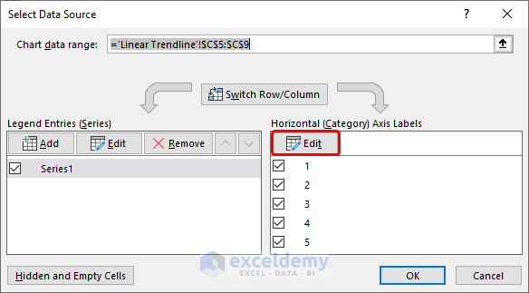
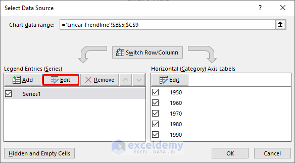
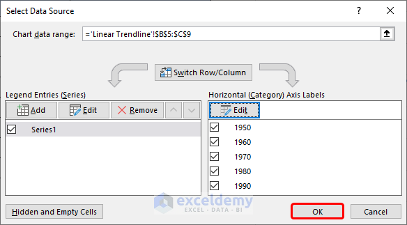
- A dialog box appears where we can change the Axis Labels to show Years. Select the Edit button under Horizontal Axis Labels.
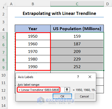
- Select the range of cells for the Years and click OK.
- Rename the series by clicking Edit on the Legend Entries section on the left.
- The Series is renamed to Actual Population.
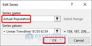
- Confirm your changes by clicking the OK and closing the dialog box.
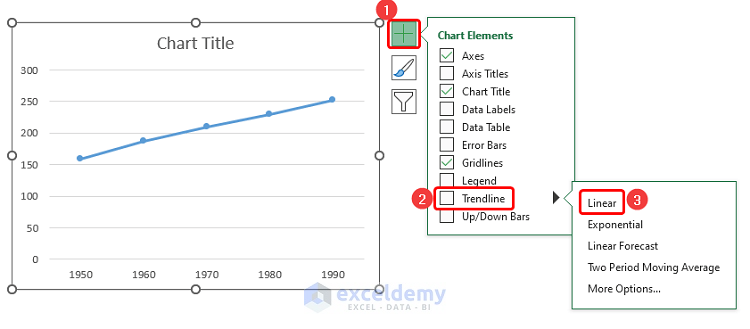
Step 3 – Insert and Format the Trendline
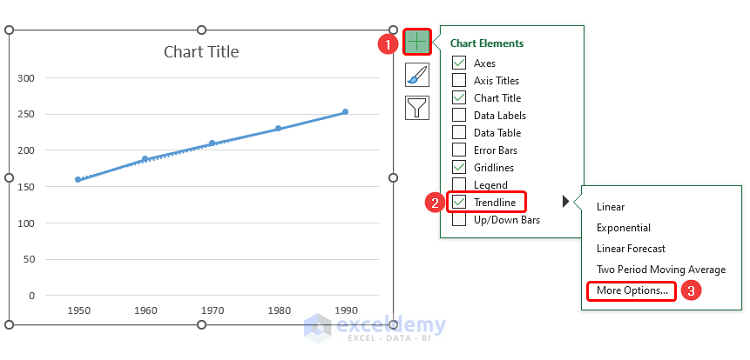
- Go to the Chart Elements and expand Trendline, then select Linear.
- Under Trendline, select More Options.
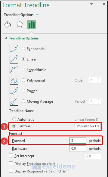
- A Format Trendline panel appears on the right. Enter a name and assign Forecast periods on our chart (Forward: 3).
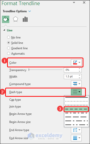
- Choose a Color and the Dash type for the trendline as shown in the picture below.
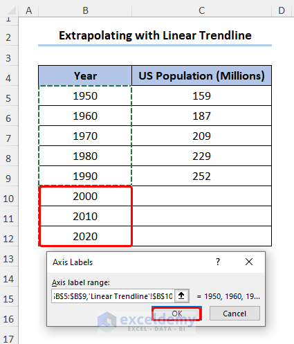
- The trendline for the next three decades appears but we have to add the Axis Labels for them.
- Go to the Data Source and select Edit for Horizonal Axis Labels.

- Hold the Ctrl key and add the remaining Years to the previous selection.
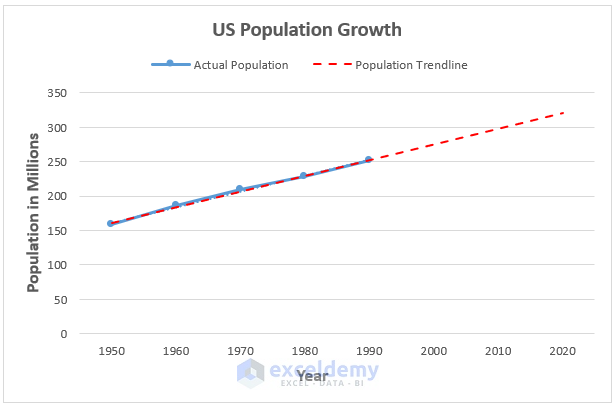
- You can edit the Axis Titles, Chart Title, and the Legend from the Chart Element option.
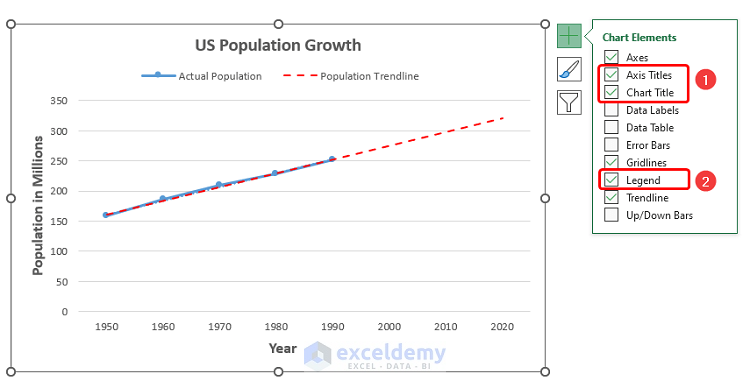
- The resulting chart should look like the picture shown below.
Method 2 – Extrapolate Non-Linear Data with a Trendline
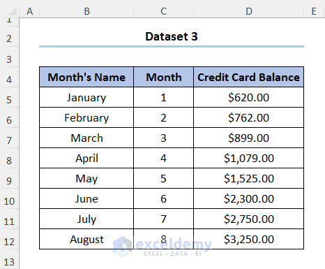
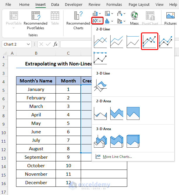
We have the following dataset shown in the B4:D12 cells below. The dataset shows the Month Name, Month numbers, and Credit Card Balance in USD. The balance doesn’t grow linearly.
Steps:
- Select the D5:D12 cells.
- Go to Insert and select Line Chart.
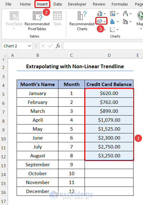
- Choose the 2D Line Chart option to represent the dataset as a line chart.
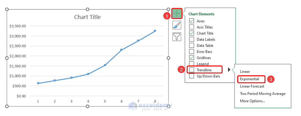
- Navigate to Chart Elements, expand Trendline, and select Exponential.
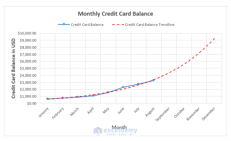
- Format the chart like in the previous method to expand the horizontal axis and add labels.
Here are the various trendline types you can find in Excel and when they’re most useful:
| Types of Trendline | Uses |
|---|---|
| Linear | A linear trendline suits a dataset that is similar to a line and where the data points change at a steady rate. |
| Exponential | An exponential trendline is useful for non-linear data where the values rise or fall at increasingly higher rates. |
| Logarithmic | A logarithmic trendline is suitable when the rate of change of values increases or decreases rapidly and then flattens out. |
| Polynomial | A polynomial trendline is handy when examining gains and losses in a large dataset. |
| Power | A power trendline matches datasets that increase at a specific rate. |
| Moving Average | A moving average trendline smoothens fluctuations by averaging a certain number of data points and using it in the trendline. |
Read More: How to Extrapolate a Graph in Excel
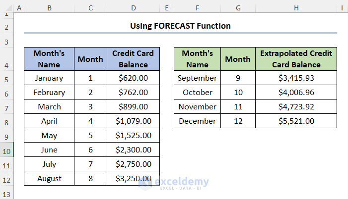
Method 3 – Extrapolate a Trendline with the FORECAST Function
Steps:
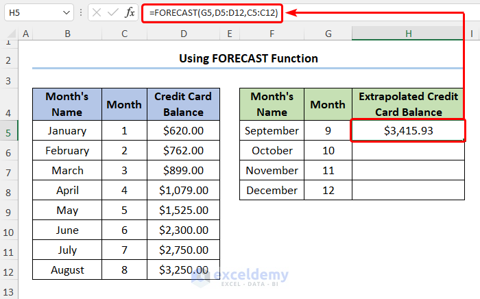
- Make a new table for calculating the extrapolated values. Our existing data is in the C5:D12 range.
- Insert the following expression given below in H5 for the first result.
=FORECAST(G5,D5:D12,C5:C12)
The G5 cell refers to the x argument while the D5:D12 and C5:C12 cells represent the known_y and known_x arguments, respectively.
- Use the Fill Handle tool to copy the formula into the cells below.
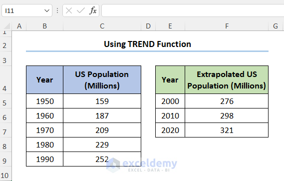
Method 4 – Extrapolate a Trendline with the TREND Function
Steps:
- We’ll use the U.S. population dataset in B5:C9.
- Create a new table in E5:F7 to store new results.
- Fill the E5:E7 range with new x-values (years you want to calculate for).
- Insert the following formula in F5.
=TREND($C$5:$C$9,$B$5:$B$9,E5)
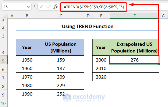
- Complete the table by copying the formula to the cells below.
Things to Remember
- The #REF! error occurs if the known_xs and the known_ys arrays have different sizes.
- The #VALUE! error is shown if you enter a non-numeric value.
- Linear extrapolation only works if the function is indeed linear. If the values don’t follow a linear progression, you can get wildly varying results.
Download the Practice Workbook
Related Articles
<< Go Back to Excel Extrapolation | Excel for Statistics | Learn Excel
Get FREE Advanced Excel Exercises with Solutions!
