In this article, we’ll discuss various methods to select rows based on cell value using VBA, along with recommended practices and potential problems. We’ll demonstrate the For…Next and Do…Loop loops, along with methods like Union, and Intersect in our VBA scripts.
How to Launch Visual Basic Editor in Excel
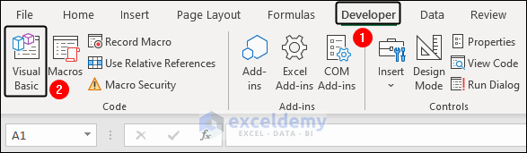
The Developer tab contains the VBA environment, including tools for creating and recording macros, Excel Add-ins, Forms controls, importing and exporting XML data, etc.
Note: By default, the Developer tab remains hidden. If you don’t see in on the ribbon, enable the Developer tab.
Steps:
- Go to the Developer tab, then click on the Visual Basic icon in the Code group.
This launches the Microsoft Visual Basic for Applications window.
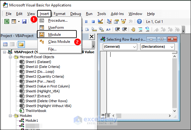
- Click on the Insert tab and choose Module from the list.
A small module window opens in which to insert our VBA code.
- After entering code, click the Run button or press the F5 key to execute the code.
The advantage of inserting the code in the module is that we can apply this code to all the worksheets in this Excel workbook. Conversely, we can make our code only available for a specific worksheet.
Excel VBA Select Row Based on Cell Value : 3 Examples
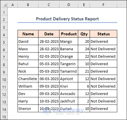
To illustrate our example, we’ll use a Product Delivery Status Report of a particular grocery store. This dataset includes the Name, Date, Product, Qty, and Status in columns B, C, D, E and F respectively.
Note: This is a basic dataset for demonstration purposes. In a practical scenario, you may encounter a much larger and more complex dataset.
We’ll select rows based on cell value using VBA using this dataset.
We used the Microsoft Excel 365 version; but you may use any other version according to your convenience. Please leave a comment if any part of this article does not work in your version.
Example 1 – Using For…Next Statement
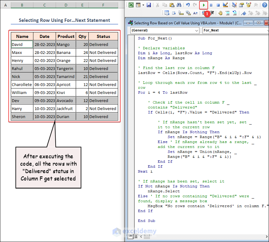
In the above image, we have selected the rows that have “Delivered” status in the F column. We use a VBA macro to accomplish this task. In the code, we use the For…Next loop, If statement, and VBA Union function. After running the code, all the desired rows (rows 5, 8, 9, 12, 14) will be selected simultaneously.
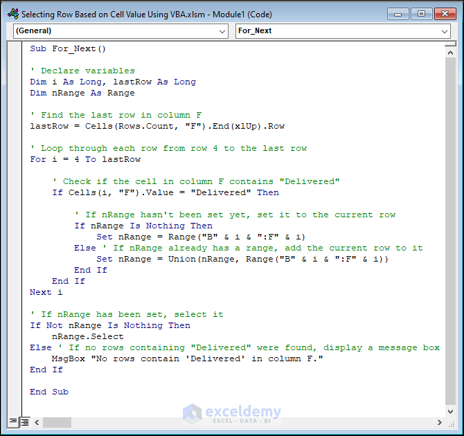
Below is the code:
Sub For_Next()
' Declare variables
Dim i As Long, lastRow As Long
Dim nRange As Range
' Find the last row in column F
lastRow = Cells(Rows.Count, "F").End(xlUp).Row
' Loop through each row from row 4 to the last row
For i = 4 To lastRow
' Check if the cell in column F contains "Delivered"
If Cells(i, "F").Value = "Delivered" Then
' If nRange hasn't been set yet, set it to the current row
If nRange Is Nothing Then
Set nRange = Range("B" & i & ":F" & i)
Else ' If nRange already has a range, add the current row to it
Set nRange = Union(nRange, Range("B" & i & ":F" & i))
End If
End If
Next i
' If nRange has been set, select it
If Not nRange Is Nothing Then
nRange.Select
Else ' If no rows containing "Delivered" were found, display a message box
MsgBox "No rows contain 'Delivered' in column F."
End If
End Sub
Code Breakdown:
- A new subroutine named For_Next is introduced.
- The variables i, lastRow, and nRange are declared and initialized next. lastRow will store the row number of the last cell containing data in Column F, and nRange is a range object.
- The Cells method and the End(xlUp) function are used to locate the last row containing data in Column F. This method is frequently used to identify the last row in a range.
- Then the For…Next loop initializes. It starts at Row 4 and iterates up to the last row just found. The loop variable i keeps track of the current row.
- The If…Then condition determines whether “Delivered” appears in Column F of the current row. If it does, the statement’s code will be executed.
- The Set statement creates a new range object for columns B to F of the current row if nRange is empty. The Union statement merges the current row’s range with any existing range objects in nRange if it already does so.
- The program verifies if nRange holds any cells once the loop has been completed. If true, the Select method is used to choose the range. If not, a message box informing the user that no rows containing “Delivered” were found is displayed.
As in the video above, whenever we execute the code, all the rows with “Delivered” status in column F are instantly selected.
Selecting rows one by one is quite simple. But showing all rows selected at once is a bit more complex because of the use of looping. The code will select a row, and at the next iteration it will select the new row that fulfills the condition. But at the same time, the previously selected row will be deselected. To display all selected rows at once, we used the VBA Union function.
Overall, this code looks for any rows in a worksheet’s column F with the value “Delivered” in them. For each such row found, it picks the range from columns B to F.
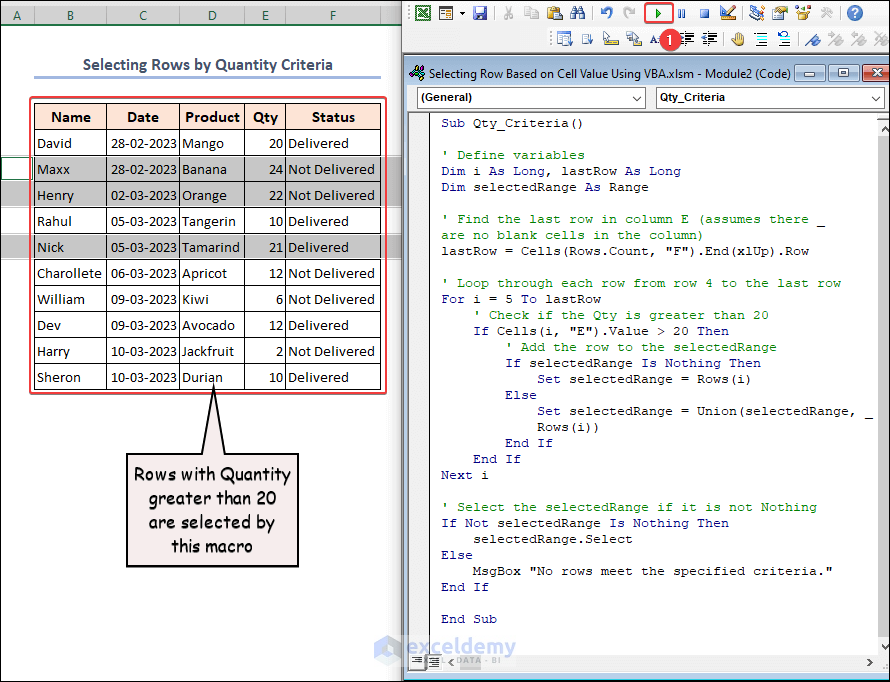
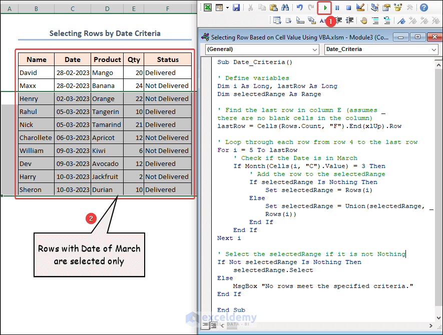
1.1 – Selecting Rows by Quantity Criteria
You may have noticed that rows containing both Delivered and Not Delivered were selected. Do you know why this happened?
In this next example, we will select rows that have sales quantities greater than 20.
Here is the code:
Sub Qty_Criteria()
' Define variables
Dim i As Long, lastRow As Long
Dim selectedRange As Range
' Find the last row in column E (assumes there are no blank cells in the column)
lastRow = Cells(Rows.Count, "F").End(xlUp).Row
' Loop through each row from row 4 to the last row
For i = 5 To lastRow
' Check if the Qty is greater than 20
If Cells(i, "E").Value > 20 Then
' Add the row to the selectedRange
If selectedRange Is Nothing Then
Set selectedRange = Rows(i)
Else
Set selectedRange = Union(selectedRange, Rows(i))
End If
End If
Next i
' Select the selectedRange if it is not Nothing
If Not selectedRange Is Nothing Then
selectedRange.Select
Else
MsgBox "No rows meet the specified criteria."
End If
End SubAs demonstrated in the video above, this code selects rows that have a quantity greater than 20 in Column E. We start the loop from Row 5 as the previous row is the heading row. As a result, rows 6, 7, and 9 are selected using the declared criteria.
The first row with data in the data table isn’t selected, because the order is for 20 mangoes, which is less than the condition. If we change our criteria in the code and alter the (>) sign to (=>) sign, then this row will also be added to the selection.
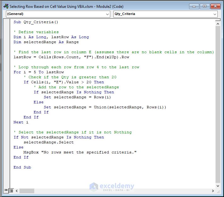
1.2 – Selecting Rows by Date Criteria
Now let’s select the rows having orders for the month of March. Rows 7 to 14 are selected, as they each have dates in March in column C. The code is almost identical to the previous method.
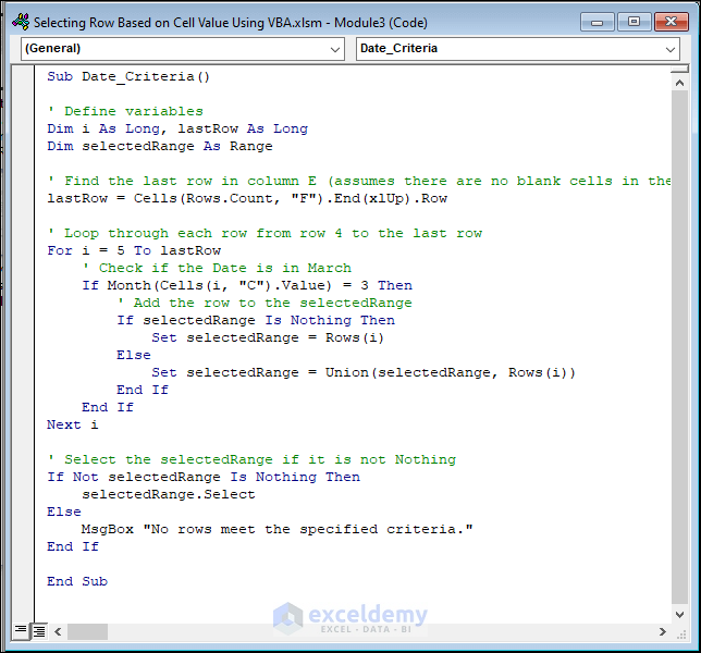
Here is the code:
Sub Date_Criteria()
' Define variables
Dim i As Long, lastRow As Long
Dim selectedRange As Range
' Find the last row in column E (assumes there are no blank cells in the column)
lastRow = Cells(Rows.Count, "F").End(xlUp).Row
' Loop through each row from row 5 to the last row
For i = 5 To lastRow
' Check if the Date is in March
If Month(Cells(i, "C").Value) = 3 Then
' Add the row to the selectedRange
If selectedRange Is Nothing Then
Set selectedRange = Rows(i)
Else
Set selectedRange = Union(selectedRange, Rows(i))
End If
End If
Next i
' Select the selectedRange if it is not Nothing
If Not selectedRange Is Nothing Then
selectedRange.Select
Else
MsgBox "No rows meet the specified criteria."
End If
End Sub
For clear understanding, read the comments in the code carefully.
As in the video above, there is another way to execute a code from the module. Instead of clicking on the Run icon in the ribbon, we can run the code using the Macro dialog box.
- Click on the Macros option in the Developer tab to open this dialog box. Alternatively, press F8 on your keyboard.
- In the Macro dialog box that opens, find the macro you created and click on the Run button in the dialog box.
After executing the code, all the rows, including the purchase orders from March, are selected at once. Generally, this code may be easily modified and applied to different Excel spreadsheets to select rows based on a certain criterion, such as a specified date range. Just alter the condition inside the If…Else statement carefully.
Example 2 – Using Do…Loop Statement
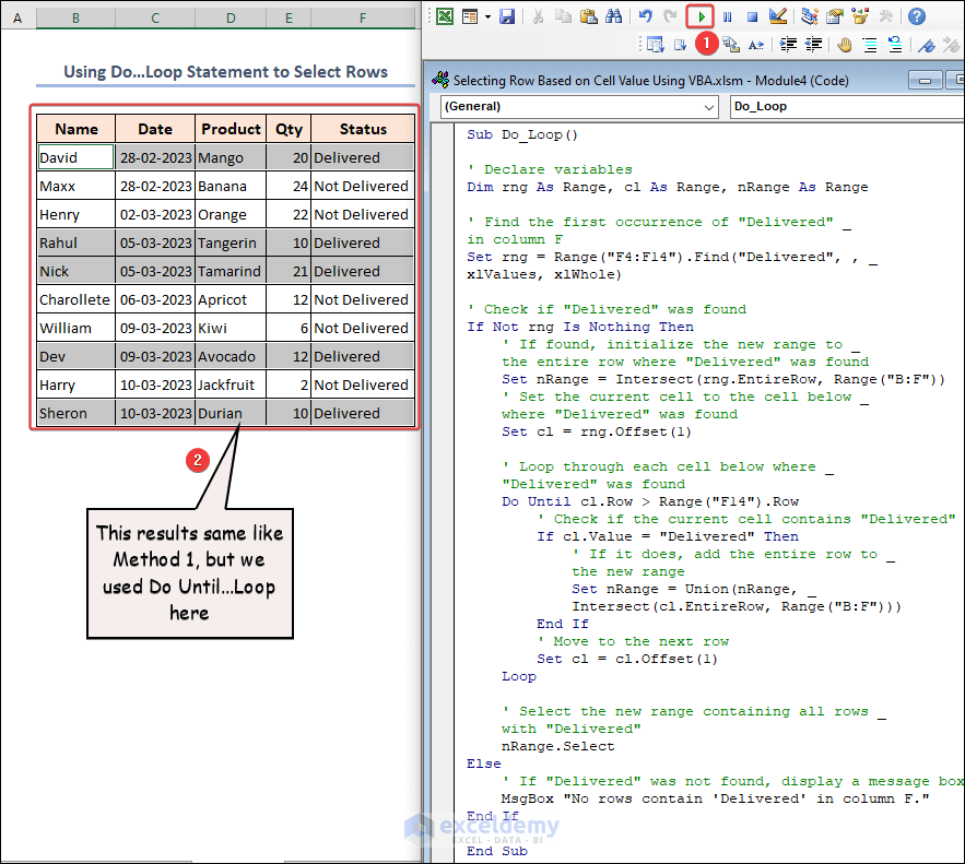
In this method, the output is the same as in Example 1. The only difference is in the code, where we use a different loop: Do…Until loop. Also, we utilize another function named the VBA Intersect function with the Union function. A message box will show the message “No rows contain “Delivered” in column F” if “Delivered” is not found in the defined range here too.
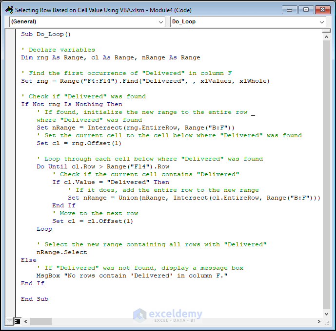
Here is the code:
Sub Do_Loop()
' Declare variables
Dim rng As Range, cl As Range, nRange As Range
' Find the first occurrence of "Delivered" in column F
Set rng = Range("F4:F14").Find("Delivered", , xlValues, xlWhole)
' Check if "Delivered" was found
If Not rng Is Nothing Then
    ' If found, initialize the new range to the entire row where "Delivered" was found
    Set nRange = Intersect(rng.EntireRow, Range("B:F"))
    ' Set the current cell to the cell below where "Delivered" was found
    Set cl = rng.Offset(1)
    ' Loop through each cell below where "Delivered" was found
    Do Until cl.Row > Range("F14").Row
        ' Check if the current cell contains "Delivered"
        If cl.Value = "Delivered" Then
            ' If it does, add the entire row to the new range
            Set nRange = Union(nRange, Intersect(cl.EntireRow, Range("B:F")))
        End If
        ' Move to the next row
        Set cl = cl.Offset(1)
    Loop
    ' Select the new range containing all rows with "Delivered"
    nRange.Select
Else
    ' If "Delivered" was not found, display a message box
    MsgBox "No rows contain 'Delivered' in column F."
End If
End Sub
Code Breakdown:
- This code will search in the range F4:F14 for the first instance of “Delivered” using the Find method. The search should look for an exact match, according to the instructions in the xlValues and xlWhole parameters. We set rng named range to the cell containing “Delivered“, if it is matched.
- The script then verifies if rng is not Nothing. If true, the code has discovered “Delivered” inside the range.
- The code initializes the new range nRange to cover only columns B through F by intersecting it with the range B:F if it has found “Delivered“. We did this by setting the EntireRow property to the full row where the code found “Delivered“. Then, it will change the current cell to the cell below where it found “Delivered“.
- Then the code starts a loop that iterates through all cells below the one where it detected “Delivered” until it reaches the last cell in the range F14.
- The code examines whether the current cell includes “Delivered” for each cell in the loop. If true, it uses the Union function and the Intersect method to include only columns B through F when adding the full row to the new range nRange.
- The code selects the new range nRange, which contains all rows with “Delivered” after the loop has finished.
It’s a good idea to have a backup plan in case something goes wrong, if possible.
In the video above, the code runs perfectly and selects all rows with “Delivered” status at once. If there are no rows with this status, the code returns a message box to confirm this.
The code can easily be modified to be used in different Excel files to choose rows based on the specific requirements.
Example 3 – Selecting Rows That Have Data in First Column
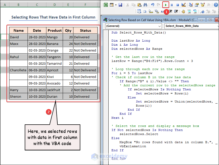
In the image above, there are some blank cells in the first column (Column B).
We’ll omit those rows that have blank cells in the first column. In other words, we’ll select those rows having values in the first column only.
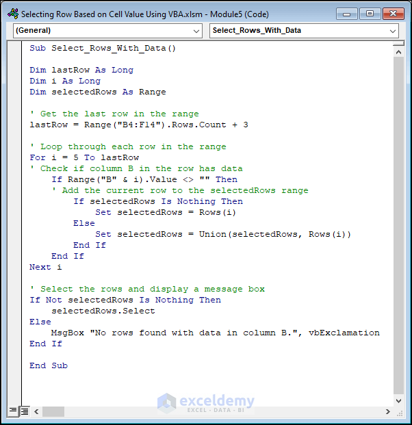
Here is the code:
Sub Select_Rows_With_Data()
Dim lastRow As Long
Dim i As Long
Dim selectedRows As Range
' Get the last row in the range
lastRow = Range("B4:F14").Rows.Count + 3
' Loop through each row in the range
For i = 5 To lastRow
' Check if column B in the row has data
If Range("B" & i).Value <> "" Then
' Add the current row to the selectedRows range
If selectedRows Is Nothing Then
Set selectedRows = Rows(i)
Else
Set selectedRows = Union(selectedRows, Rows(i))
End If
End If
Next i
' Select the rows and display a message box
If Not selectedRows Is Nothing Then
selectedRows.Select
Else
MsgBox "No rows found with data in column B.", _
vbExclamation
End If
End SubAfter executing the code, the first two rows are selected, but not the third, because it doesn’t have any value in cell B7. We again started the loop from row 5 to ignore the heading row.
Read More: Excel VBA to Select Last Row
How to Highlight Row Based on Cell Value Using VBA
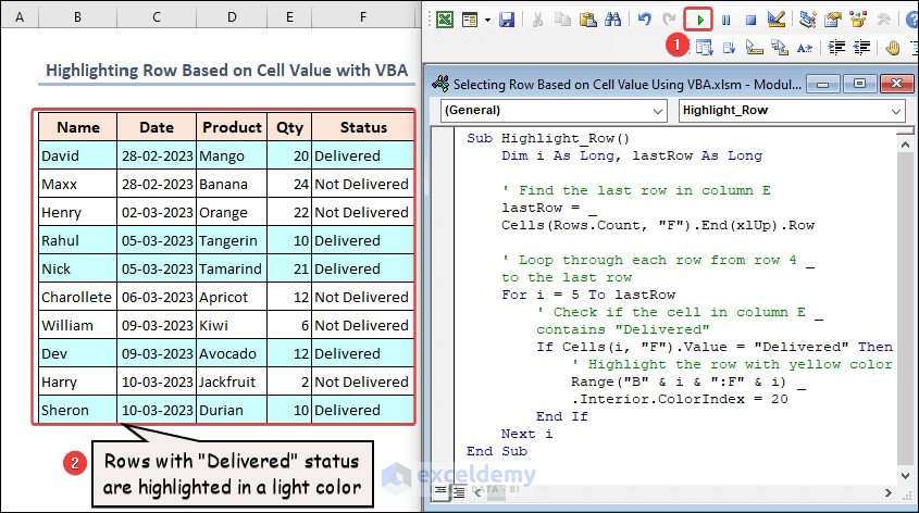
Now we’ll highlight the rows that have “Delivered” status in Column F with a light background fill color. It is a simpler process to highlight rows than select them using VBA.
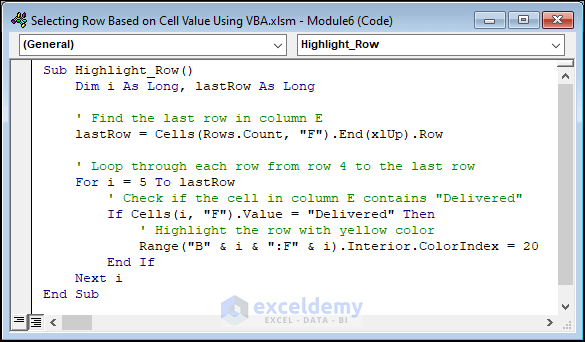
Here is the code:
Sub Highlight_Row()
Dim i As Long, lastRow As Long' Find the last row in column E
lastRow = Cells(Rows.Count, "F").End(xlUp).Row' Loop through each row from row 4 to the last row
For i = 5 To lastRow
' Check if the cell in column E contains "Delivered"
If Cells(i, "F").Value = "Delivered" Then
' Highlight the row with yellow color
Range("B" & i & ":F" & i).Interior.ColorIndex = 20
End If
Next i
End Sub
Although more complex, we can also use a modified version of the code we used in Method 2. We have to change just a property.
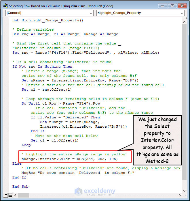
Sub Highlight_Change_Property()
' Define variables
Dim rng As Range, cl As Range, nRange As Range
' Find the first cell that contains the value "Delivered" in column F (range F4:F14)
Set rng = Range("F4:F14").Find("Delivered", , xlValues, xlWhole)
' If a cell containing "Delivered" is found
If Not rng Is Nothing Then
' Define a range (nRange) that includes the entire row of the found cell, but only columns B:F
Set nRange = Intersect(rng.EntireRow, Range("B:F"))
' Define a variable for the cell directly below the found cell
Set cl = rng.Offset(1)
' Loop through the remaining cells in column F (down to F14)
Do Until cl.Row > Range("F14").Row
' If a cell contains "Delivered", add the entire row (but only columns B:F) to the nRange range
If cl.Value = "Delivered" Then
Set nRange = Union(nRange, _
Intersect(cl.EntireRow, Range("B:F")))
End If
' Move to the next cell below
Set cl = cl.Offset(1)
Loop
' Highlight the entire nRange range in a light color
nRange.Interior.Color = RGB(254, 253, 195)
Else
' If no cells containing "Delivered" are found, display a message box
MsgBox "No rows contain 'Delivered' in column F."
End If
End Sub
Just after the Do…Until loop, we change the property of the range named nRange from Select to Interior.Color. With this little change, we highlight the rows with the color matching the specified RGB code.
As in the video, the code highlights the rows with “Delivered” status with a light background color (pastel yellow).
Due to its relative simplicity, we recommend using the first method to highlight rows.
How to Extract Row Based on Cell Value Using VBA in Excel
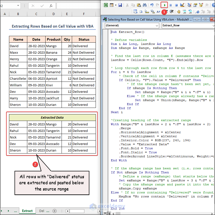
Now we will extract the rows with “Delivered” status, and paste them into a new range (B16:F21) just below the source range.
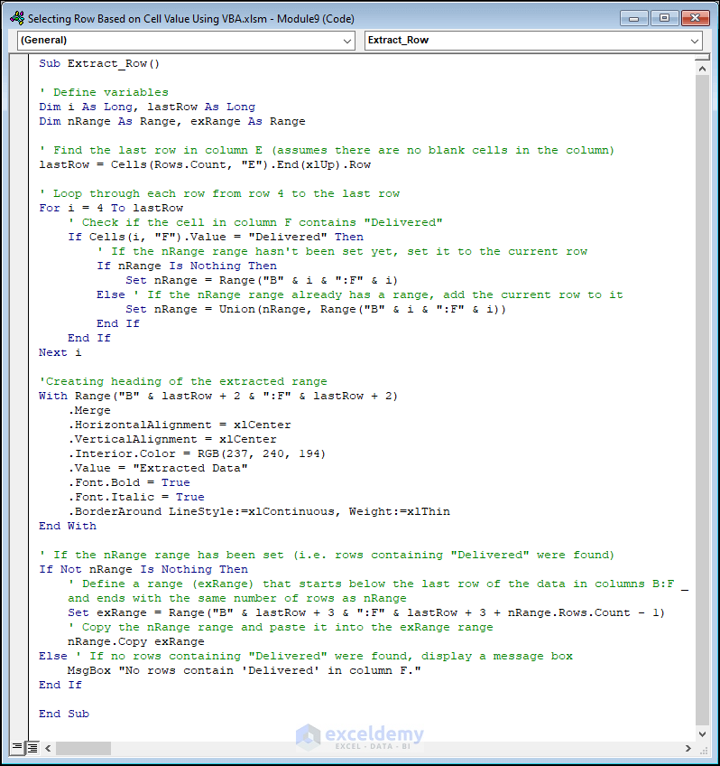
Here is the code:
Sub Extract_Row()
' Define variables
Dim i As Long, lastRow As Long
Dim nRange As Range, exRange As Range
' Find the last row in column E (assumes there are no blank cells in the column)
lastRow = Cells(Rows.Count, "E").End(xlUp).Row
' Loop through each row from row 4 to the last row
For i = 4 To lastRow
    ' Check if the cell in column F contains "Delivered"
    If Cells(i, "F").Value = "Delivered" Then
        ' If the nRange range hasn't been set yet, set it to the current row
        If nRange Is Nothing Then
            Set nRange = Range("B" & i & ":F" & i)
        Else ' If the nRange range already has a range, add the current row to it
            Set nRange = Union(nRange, Range("B" & i & ":F" & i))
        End If
    End If
Next i
'Creating heading of the extracted range
With Range("B" & lastRow + 2 & ":F" & lastRow + 2)
    .Merge
    .HorizontalAlignment = xlCenter
    .VerticalAlignment = xlCenter
    .Interior.Color = RGB(237, 240, 194)
    .Value = "Extracted Data"
    .Font.Bold = True
    .Font.Italic = True
    .BorderAround LineStyle:=xlContinuous, Weight:=xlThin
End With
' If the nRange range has been set (i.e. rows containing "Delivered" were found)
If Not nRange Is Nothing Then
    ' Define a range (exRange) that starts below the last row of the data in columns B:F and ends with the same number of rows as nRange
    Set exRange = Range("B" & lastRow + 3 & ":F" & lastRow + 3 + nRange.Rows.Count - 1)
    ' Copy the nRange range and paste it into the exRange range
    nRange.Copy exRange
Else ' If no rows containing "Delivered" were found, display a message box
    MsgBox "No rows contain 'Delivered' in column F."
End If
End Sub
Follow the comments to understand the code.
As illustrated in the video, after running the code a source range is visible in the worksheet. The rows matching the criterion are extracted and placed in a range below one row of the main data table. If you run the code again, delete the range with extracted data first.
How to Delete All Other Rows Based on Cell Value with VBA
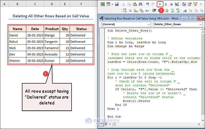
The next code segment will delete all other rows except those with “Delivered” status.
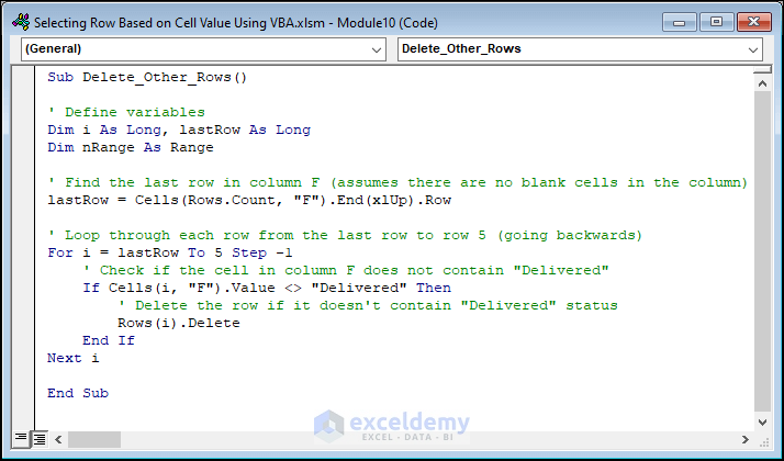
Here is the code:
Sub Delete_Other_Rows()
' Define variables
Dim i As Long, lastRow As Long
Dim nRange As Range
' Find the last row in column F (assumes there are no blank cells in the column)
lastRow = Cells(Rows.Count, "F").End(xlUp).Row
' Loop through each row from the last row to row 5 (going backwards)
For i = lastRow To 5 Step -1
' Check if the cell in column F does not contain "Delivered"
If Cells(i, "F").Value <> "Delivered" Then
' Delete the row if it doesn't contain "Delivered" status
Rows(i).Delete
End If
Next i
End SubWhen we run the code, all rows except those with “Delivered” status are removed from the sheet. After each row is deleted, the row below it moves up and fills the empty space.
How to Highlight Rows with Different Colors Based on Multiple Criteria Without VBA
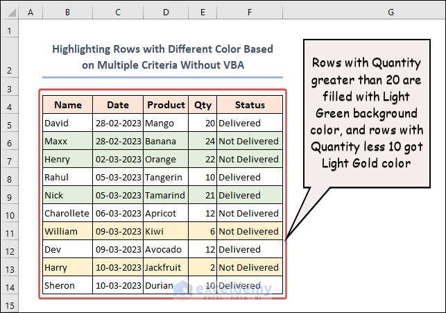
Now we’ll set a Conditional Formatting rule for the table such that it will highlight rows with values greater than 20 in the ‘Qty‘ column with a light green background color, and rows with values less than 10 in the ‘Qty‘ column with a light gold background color. Any rows in the table that do not meet either of the criteria specified will retain their original formatting and will not have a fill color applied to their background.
Steps:
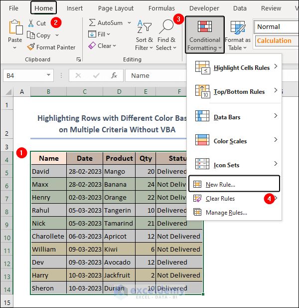
- Select the data range to apply the Conditional Formatting.
- Select Home >> Conditional Formatting >> New Rule.
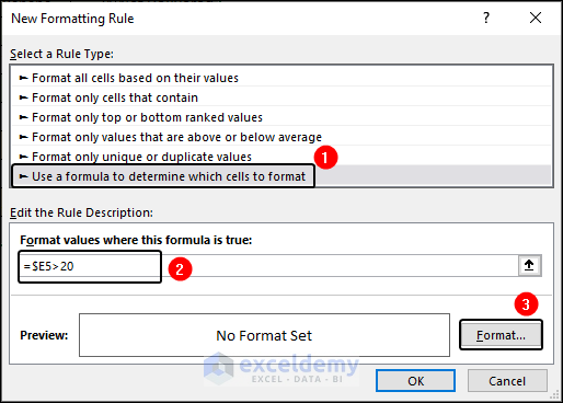
- The New Formatting Rule dialog box will appear.
- Click on Use a formula to determine which cells to format.
- Enter the below formula in the box:
=$E5>20- Click on the Format button.
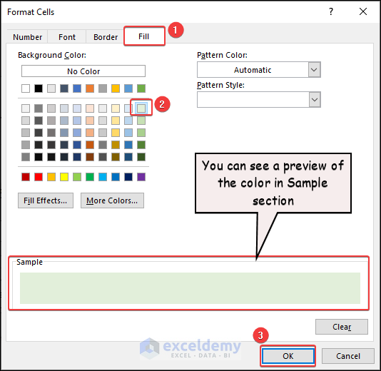
- In the Format Cells dialog box, click the Fill tab, where the desired background color will be selected.
- Choose a color as shown in the above image and click OK.
- In the New Formatting Rule dialog box, just click on the OK button again to apply the formatting and exit the dialog box.
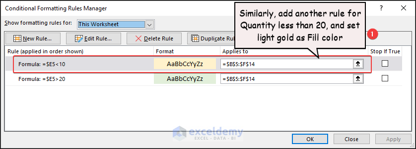
- In a similar way, add a new rule giving those rows with a quantity less than 10 a light gold background color.
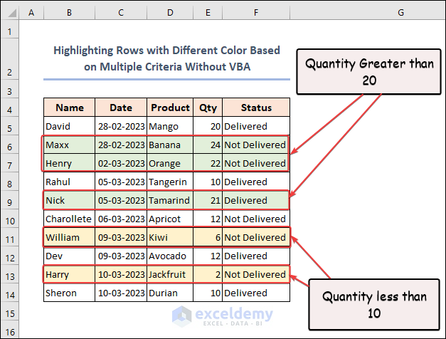
The two rules are successfully applied in the worksheet, but there is no effect of these rules on other sheets. If we change the value of the quantity in any row, then if it meets the criteria, the row color will automatically change. Suppose you change the order quantity of David from 20 to 25. What will the fill color of Row 5 be? Let us know in the comment section.
Frequently Asked Questions
- What happens if there are numerous cells in the range that have the same value?
All the methods in our reference cover this possibility. We have several rows with the same value in a respective column, and we select all those rows which have the specific value in that particular column.
- Is it possible to select a row using multiple cell values?
You can change the code to choose a row depending on a variety of cell values. Using numerous If statements to verify each column in the row for the desired values is one approach to accomplishing this. Using the AND statement is another. In Method 1.1 and Method 1.2, we showed how we can select rows by quantity criteria and date criteria in two different sheets. To do this in a single method, you’ll have to write a code to select rows that have Quantity greater than 20 and whose Dates are in March month. If you can, let us know in the comment section.
- Is it possible to select a range of cells based on a cell value?
Use a similar piece of code to select a range of cells depending on a cell value. You would choose the range of cells that contain the corresponding value rather than choosing the full row. Also, you can accomplish this by changing the Row property in the code to the Range property.
- If the value you’re looking for is not inside the range, what should you do?
The code won’t select any rows if the value you’re looking for isn’t available in the range. You can incorporate an error handler that informs the user that the code did not find the value to deal with this situation. In our codes, we added a part to show a message box with the message “No rows contain “Delivered” in Column F” in the Else part of the If statement.
- Can I use this code for a filtered range?
Yes. But you must make sure that you have included both visible and hidden cells in the search range. You can accomplish this by either utilizing the complete column range for the search or the SpecialCells method to pick only visible cells.
Things to Remember
- Your dataset’s size will determine whether you need to optimize the code to boost performance. You can achieve this by reducing the number of times you enter the worksheet and removing unnecessary calculations or loops.
- Always select the range before applying Conditional Formatting as this sets the range of applications.
- Make sure to put an equal sign “=” before the formula in the New Formatting Rule dialog box. Otherwise, it won’t work.
- If you delete rows with VBA code, you cannot undo this action and make them visible again by just pressing CTRL + Z.
Download Practice Workbook
Get FREE Advanced Excel Exercises with Solutions!
