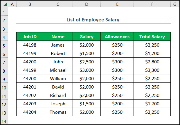
Consider the List of Employee Salary dataset shown in the B4:F13 cells containing the Job ID, Name, Salary, Allowances, and Total Salary columns, respectively. We want to display the formula used to obtain the Total Salary.
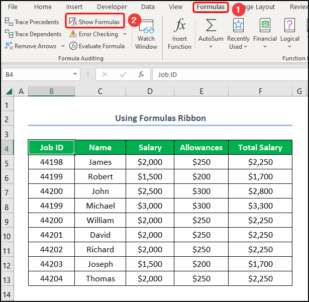
Method 1 – Using the Formulas Ribbon
Steps:
- Go to the Formulas ribbon and click the Show Formulas button.
Note: We can also use the CTRL + ` (Tilde) keys to show the formulas.
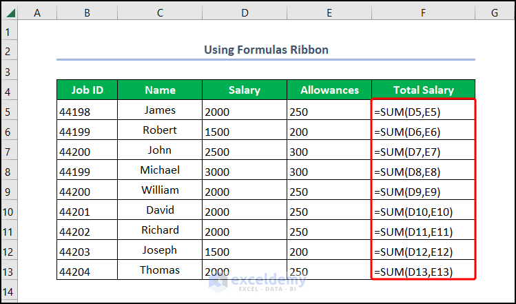
Here’s the result.
Note: When using this method, Excel automatically changes the text alignment and the column width.
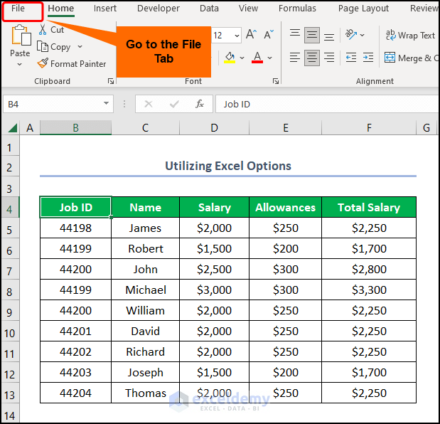
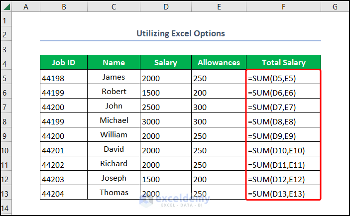
Method 2 – Utilizing Excel Options
Steps:
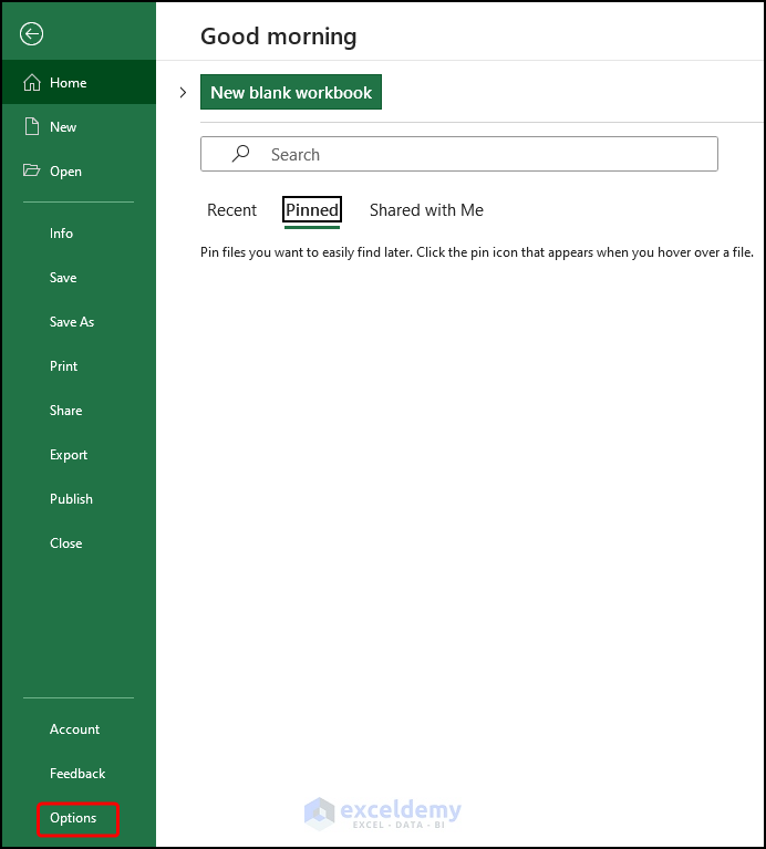
- Click the File tab located at the top-left corner.
- Press the Options button at the bottom.
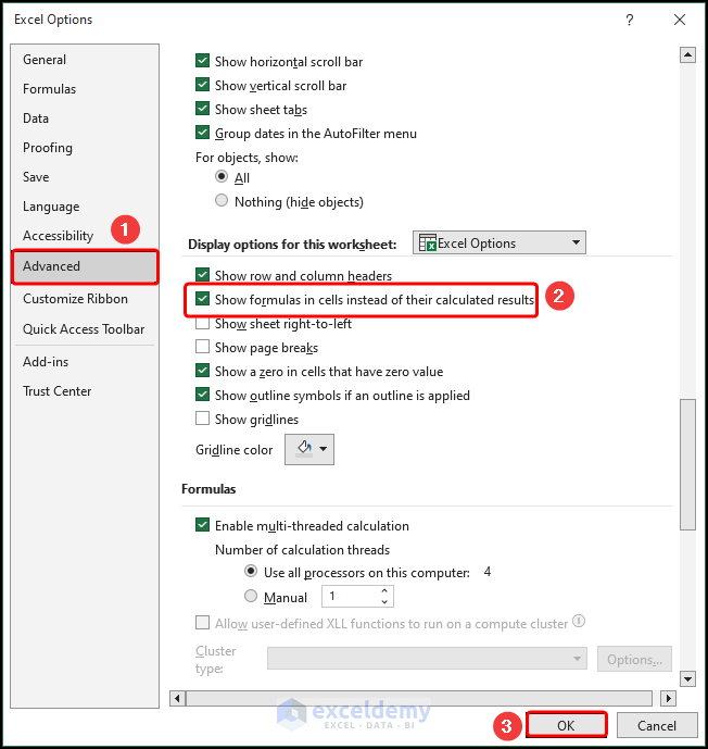
- Move to the Advanced tab.
- Scroll down to the Display options for this worksheet section.
- Check Show formulas in cells instead of their calculated results.
- Hit OK.
The results should resemble the image shown below.
Note: By default, Excel automatically increases the column width and changes the text alignment.
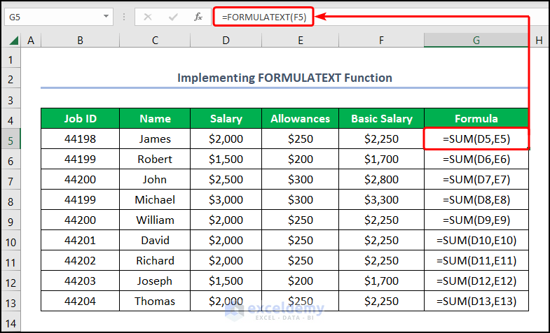
Method 3 – Implementing the FORMULATEXT Function
Steps:
- Go to the G5 cell and enter the formula given below.
=FORMULATEXT(F5)
The F5 cell refers to the Basic Salary of James.
- Drag the Fill Handle tool down to copy the formula to the cells below.
Method 4 – Applying Find & Select
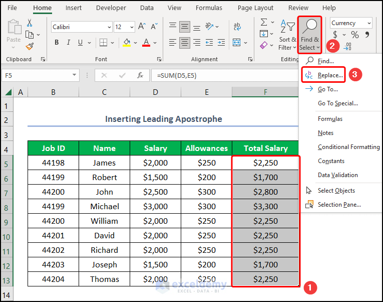
Case 4.1 – Inserting a Leading Apostrophe
Steps:
- Select the F5:F13 cells.
- Navigate to the Find & Select drop-down.
- Choose the Replace option.
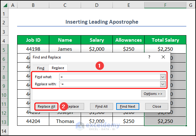
- In the Find what field, enter an Equal sign.
- In the Replace with field, type a leading Apostrophe and then an Equal sign.
- Hit Replace All.
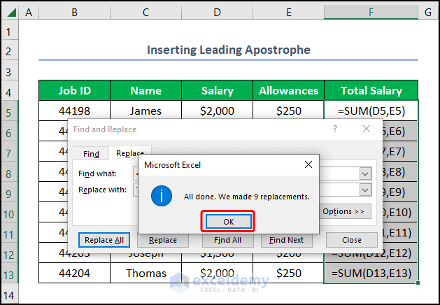
- Click OK to close the alert.
- Hit Close.
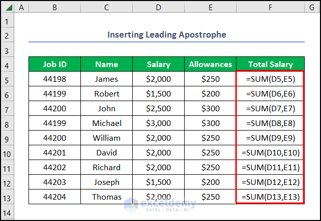
The results should look like the picture given below.
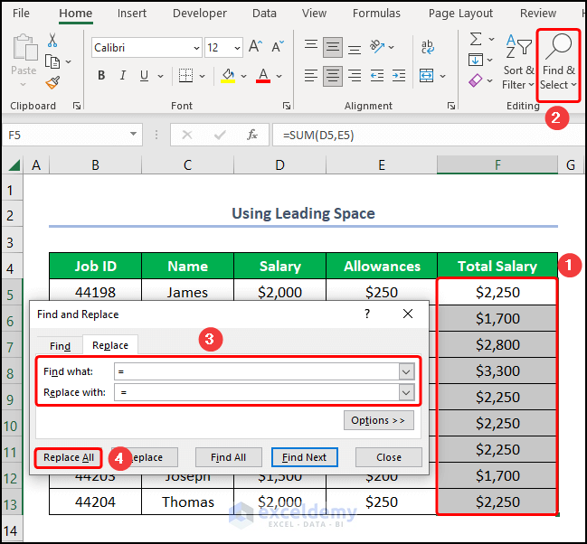
Case 4.2 – Using a Leading Space
Steps:
- Select the F5:F13 cells.
- Proceed to Find & Select, then choose the Replace option.
- In the Find what box, put an equals sign.
- In the Replace with field, put a space and an equals sign.
- Press Replace All.
- Confirm and close the dialog.
Note: You can also press the Ctrl + H keys to directly open the Find & Replace dialog box.
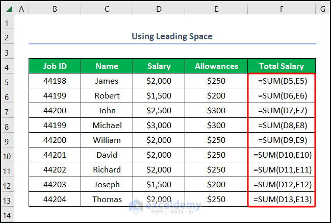
The final output should appear in the screenshot below.
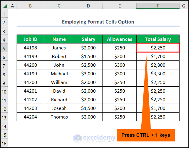
Method 5 – Employing the Format Cells Option
Steps:
- Go to the F5 cell and hit the Ctrl + 1 shortcut.
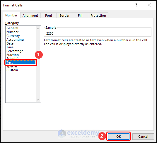
- In the Format Cells window, select the Text tab and click on OK.
- Move to the F5 cell and press the F2 key, then hit Enter key.
- Repeat the same process for the cells below.
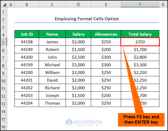
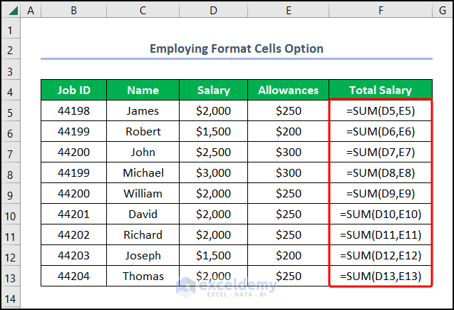
The result should look like the figure given below.
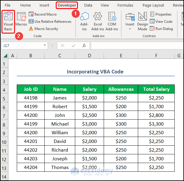
Method 6 – Incorporating VBA Code
Steps:
- Navigate to the Developer tab and click the Visual Basic button.
- Go to the Insert tab and select Module.
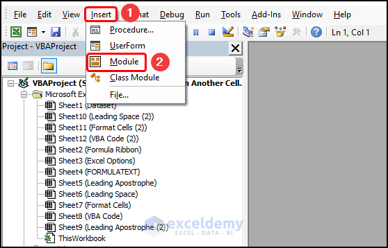
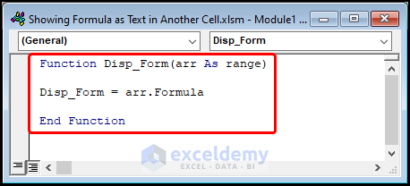
- Copy the code from here and paste it into the window as shown below.
Function Disp_Form(arr As range)
Disp_Form = arr.Formula
End Function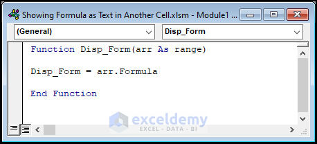
- The name of the subroutine is Disp_Form()
- We defined the argument arr and assign it as Range.
- We used the Range.Formula property to display the formulas as text.
- Close the VBA window.
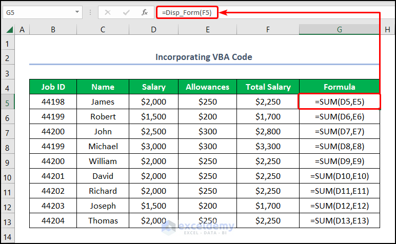
- Go to the G5 cell and call the Disp_Form function.
=Disp_Form(F5)
The F5 cell represents James’s Basic Salary.
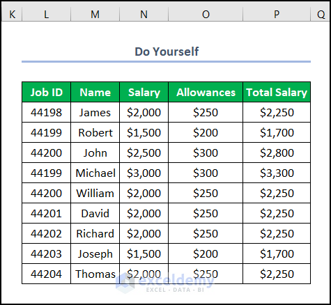
Practice Section
We have provided a Practice section on the right side of each sheet so you can practice.
Download the Practice Workbook
Related Articles
- How to Display Cell Formulas in Excel
- How to Show All Formulas in Excel
- Why Excel Shows Formulas Instead of Results
- How to Show Formula in Cells Instead of Value in Excel
- How to Show Value Instead of Formula in Excel
- How to Show Formulas When Printing in Excel
- [Fixed!] Formula Result Showing 0 in Excel
<< Go Back To Show Excel Formulas | Excel Formulas | Learn Excel
Get FREE Advanced Excel Exercises with Solutions!
