How to Generate Random Number from List in Excel (4 Ways)

Method 1 – Using INDEX and RANDBETWEEN Functions to Get a Random Number from a List in Excel

In the following picture, Column B has ten integer values in sequential order. In Cell D5, we’ll extract a random number from the list.

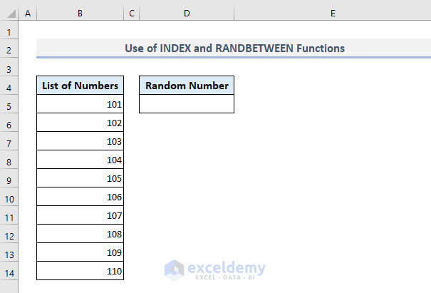
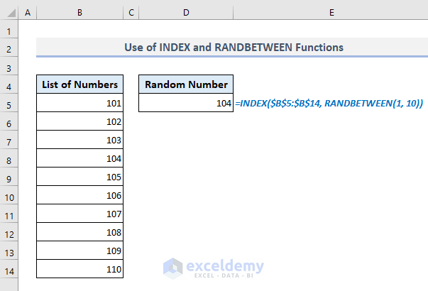
The required formula in the output Cell D5 will be:

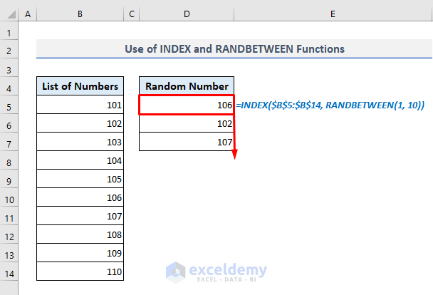
=INDEX($B$5:$B$14, RANDBETWEEN(1, 10))

After pressing Enter, the formula will return any of the numbers from the list in Column B.

If you want to get more random numbers, use the Fill Handle option to fill down from Cell D5. You’ll get more random numbers in Column D and some of them may appear as repeated values.

Method 2 – Using INDEX, RANDBETWEEN, and ROWS Functions to Get a Random Number from a List

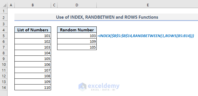
The ROWS function will count the number of rows present in the range of cells B5:B14 and assign the counted value to the upper limit of the RANDBETWEEN function.

The formula in Cell D5 is:

=INDEX($B$5:$B$14,RANDBETWEEN(1,ROWS(B5:B14)))

After pressing Enter and auto-filling a few cells under D5, you’ll be shown random outputs.

You can use the COUNTA function instead of the ROWS function:

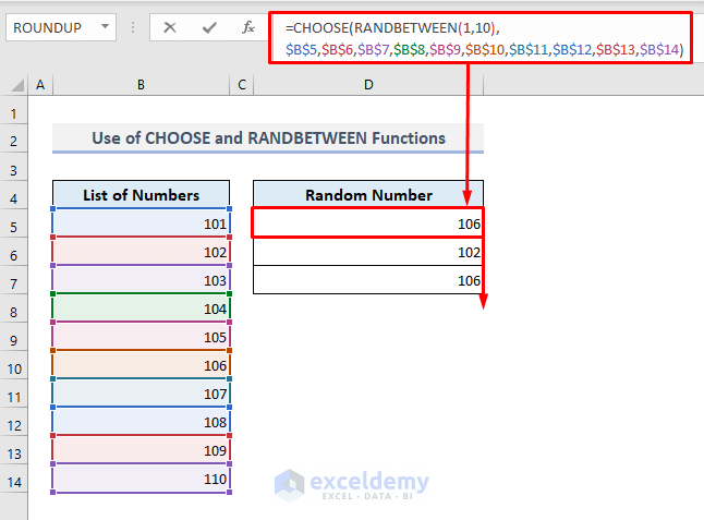
=INDEX($B$5:$B$14,RANDBETWEEN(1,COUNTA(B5:B14)))

Method 3 – Combining CHOOSE and RANDBETWEEN Functions to Extract Random Numbers from a List

In Cell D5, the required formula is:

=CHOOSE(RANDBETWEEN(1,10),$B$5,$B$6,$B$7,$B$8,$B$9,$B$10,$B$11,$B$12,$B$13,$B$14)

After pressing Enter and filling down some other cells, you’ll get the random numbers as shown in the following screenshot.

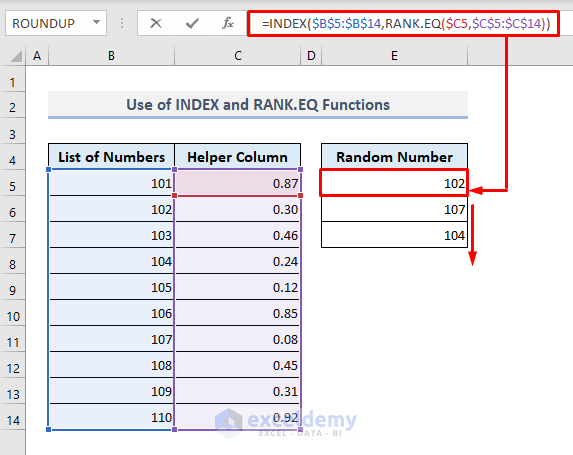
Method 4 – Generating a Random Number from a List with INDEX and RANK.EQ Functions in Excel

This method doesn’t repeat the values.
Create a helper column in Column C with the RAND function. The RAND function will return the random decimal values between 0 and 1. The RANK.EQ function will rank these decimal values in ascending or descending order. Unless you specify the order, the function will rank the values in descending order.
The required formula in the output Cell E5 will be:

=INDEX($B$5:$B$14,RANK.EQ($C5,$C$5:$C$14))

Press Enter, autofill some of the other cells under E5 and you’ll get the random values from Column B.
You’ll be able to fill down the cells up to E14. If you go beyond E14, the cells will show #N/A errors.