We may create relationships between multiple columns and rows in a PivotTable. We can examine data in multiple columns for the same values. Furthermore, we may compute Subtotals for individual parts if desired. In this tutorial, we will show you how to subtotal multiple columns in Excel Pivot Table.
How to Subtotal Multiple Columns in Excel Pivot Table: with Easy Steps
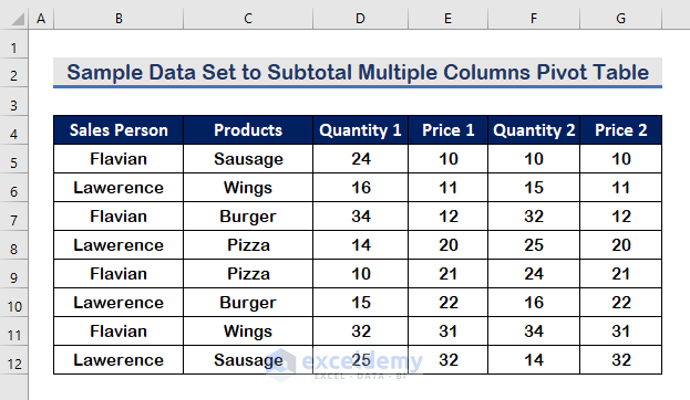
We have given a data collection comprising the sales details of two Sales Persons in the image below. For example, we want to obtain the Subtotalsof multiple columns for various categories such as Quantity 1, Quantity 2, Price 1, and Price 2. To do this, we will use our current data collection to construct a Pivot Table. Later on, we will use PivotTable Features to calculate the subtotal of multiple columns.
Step 1: Create a Pivot Table in Excel
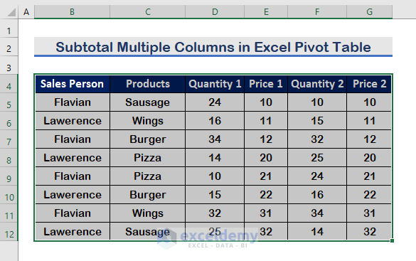
- To create a Pivot Table, select the data set with the Column Header.
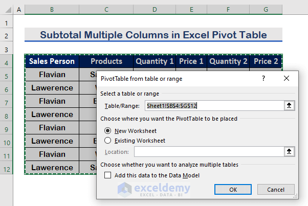
- Click on the Insert tab.
- Then, select the PivotTable option.

- Mark the New Worksheet option.
- Finally, press Enter to create PivotTable.
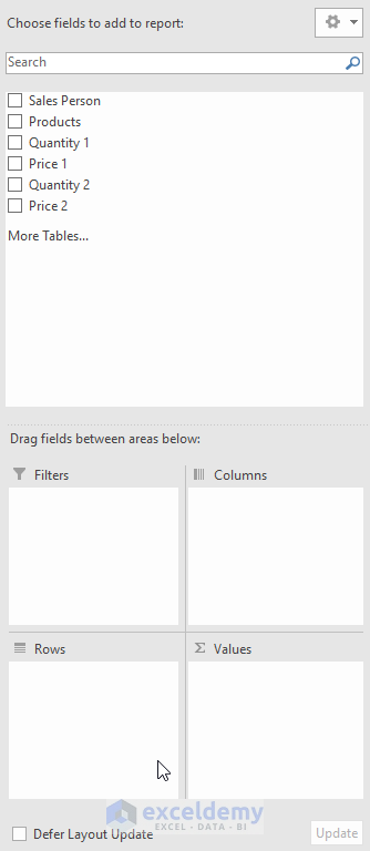
- Therefore, your PivotTable will be created in a new worksheet. The PivotTable Fields will show as the image shown below.
Step 2: Find the Subtotal of Multiple Columns in Excel Pivot Table for Each Sales Person
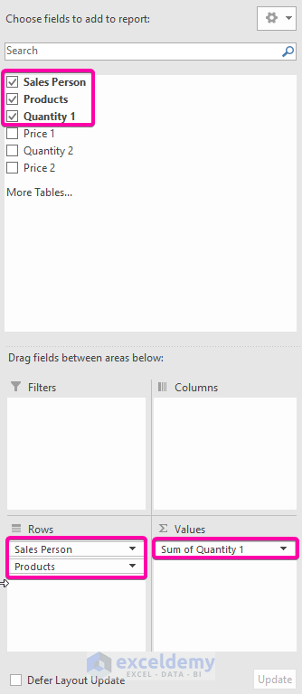
- Firstly, we will calculate the subtotal of Quantity 1 for different Products. So, select the three following options to show in the Pivot Table.
- Put the Sales Person into the Rows section at first. The first element in the Rows is the Outer Field. Subtotal will show results only for the Outer Fields.
- Then, put the Products into the Rows section as the Inner Field.
- Finally, place Quantity 1 in the Values section for which it will calculate the subtotal.
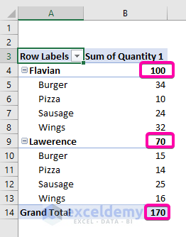
- As a result, it will show the subtotals of Quantity 1 for each Sales Person.
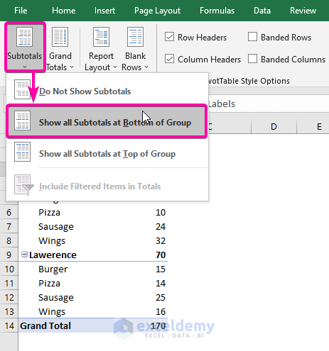
- To show all the subtotals at bottom of each group, click on the Subtotals option from the Design
- Then, select the Show all Subtotals at Bottom of Group option from the list.
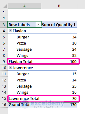
- Consequently, the subtotals will appear at the bottom of each group.
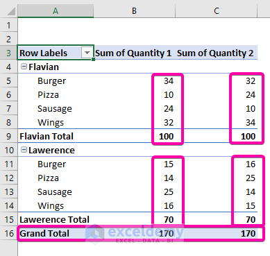
- Add another column Quantity 2 in the Values section, to subtotal the Quantity 2 for each Sale Person.
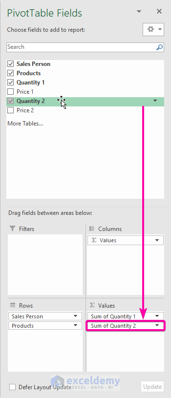
- Therefore, the subtotal of Quantity 2 column will show in the image shown below.
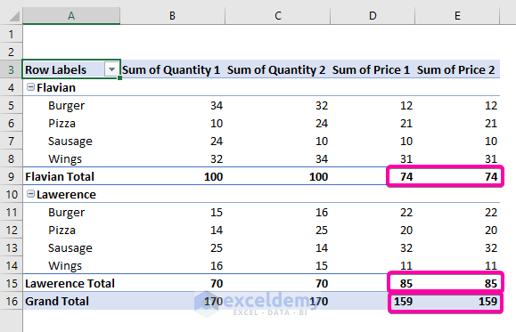
- Finally, add the rest two columns Price 1 and Price 2 in the Values section to show the subtotals of these two columns.
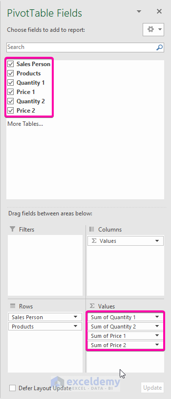
- As a consequence, all the subtotals of the columns in our data set will appear as in the image shown below.
Step 3: Calculate the Subtotal of Multiple Columns in Excel Pivot Table for Each Product
- On the other hand, to calculate the subtotals of multiple columns for each Product, place the Product in the first place in the Rows.
- Click on the Products and select the Move Up command.
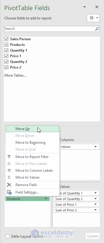
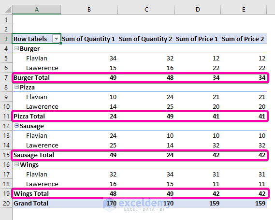
- Therefore, it will show results for each Product with the subtotals of the 4 columns.
Step 4: Summarize the Subtotal in a Particular Formation
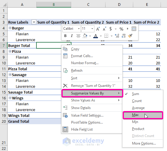
- You may also summarize the Subtotal value using any specific format, such as Maximum(Max), Minimum(Min), Average, Product, or Count
- Right-click the Subtotal cell.
- Click on the Summarize Values By.
- Then, select the Max option to show the maximum values.
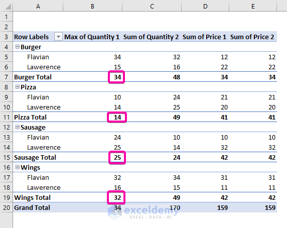
- Finally, the maximum values of Quantity 1 will be shown as seen in the image below.
Read More: How to Remove Subtotal in Pivot Table
Download Practice Workbook
Download this practice workbook to exercise while you are reading this article.
Conclusion
To conclude, I hope this article has given you some useful information about how to subtotal multiple columns in an Excel pivot table. All of these procedures should be learned and applied to your dataset. Take a look at the practice workbook and put these skills to the test. We’re motivated to keep making tutorials like this because of your valuable support.
If you have any questions – Feel free to ask us. Also, feel free to leave comments in the section below.
<< Go Back to Subtotals in Pivot Table | Pivot Table Calculations | Pivot Table in Excel | Learn Excel
Get FREE Advanced Excel Exercises with Solutions!
