How to Remove Subtotal in Pivot Table (5 Useful Ways)

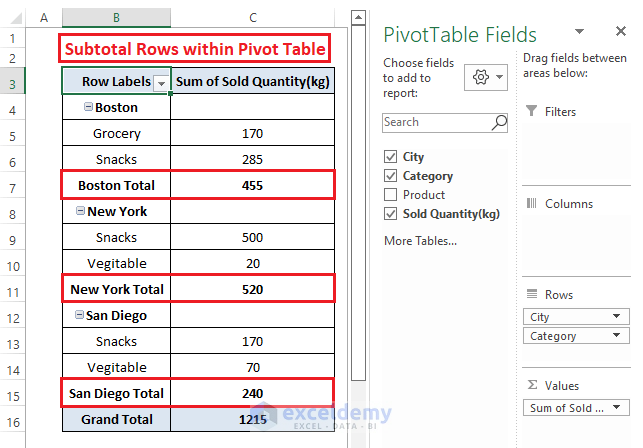
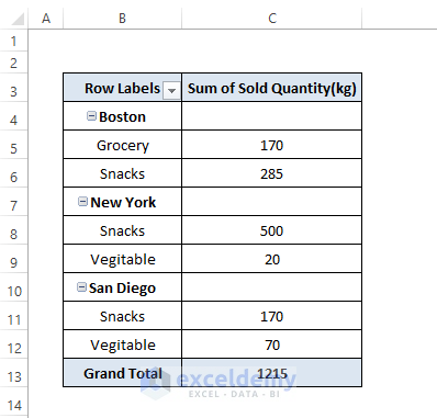
Here we have a Pivot Table that shows subtotals for various categories. We’ll remove these subtotals.

How to Remove the Subtotal in a Pivot Table: 5 Easy Ways

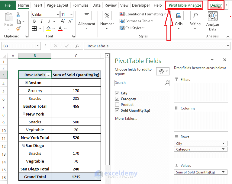
While working with a Pivot Table, Excel shows PivotTable Analyze and Design tab in the ribbon and multiple options to alter Fields, Display, or Orientation. We’ll use these two tabs to remove the Subtotal entries.

Method 1 – Using the Pivot Table Design Tool to Remove Subtotals

Steps:

• Go to Design.
• Click on Subtotal.
• Select Do Not Show Subtotals (from the Subtotal options).

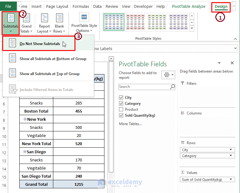
• Excel removes all the Subtotal fields from the Pivot Table as shown in the picture.

Method 2 – Remove Subtotal by Deselecting the Context Menu Option

Steps:

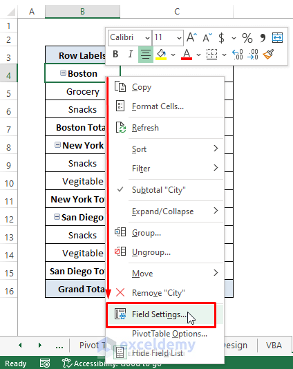
• Right-click on any City entry.
• The Context Menu appears.
• From the Context Menu, deselect the Subtotal City option.

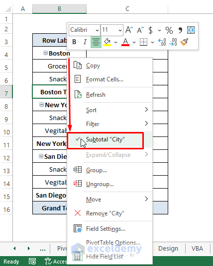
• Excel removes Subtotal fields from the Pivot Table.

Method 3 – Remove the Subtotal in a Pivot Table Using the Field Setting Options

Steps:

• Select the PivotTable Analyze tab.
• Click on Field Setting (in the Active Field section).

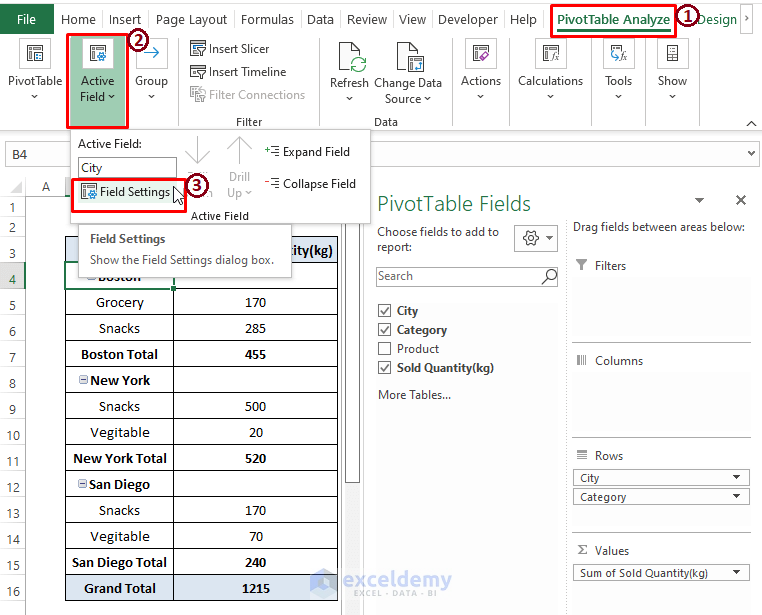
Alternatively, you can right-click on any City cell entries (i.e., Subtotals) to bring out the Context Menu and choose Field Setting. Otherwise, Excel displays Value Field Setting if you right-click on Value entries.

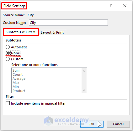
• The Field Setting window appears.
• Choose the Subtotals & Filters section (in case Excel automatically doesn’t select it).
• Under Subtotals, mark None.
• Click on OK.

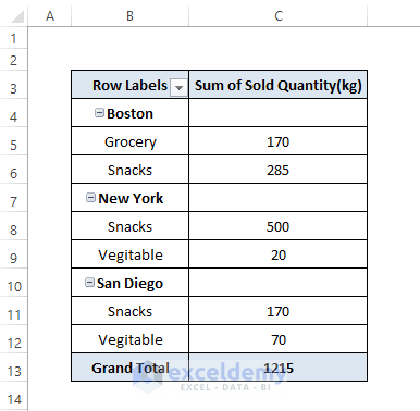
• Excel displays all the fields except the Subtotal of the Cities in the Pivot Table.

Method 4 – Using VBA Macro to Remove Subtotals in a Pivot Table

Steps:

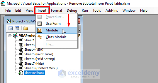
• Use Alt + F11 or go to the Developer tab and select Visual Basic (in the Code section) to open Microsoft Visual Basic window.
• Click on Insert.
• Select Module to insert a Module.

• Paste the below macro in the Module.

Sub SubtotalRemoval()
Dim mPT As PivotTable
Dim mPF As PivotField
On Error Resume Next
For Each mPT In Application.ActiveSheet.PivotTables
For Each mPF In mPT.PivotFields
mPF.Subtotals(1) = True
mPF.Subtotals(1) = False
Next
Next
End Sub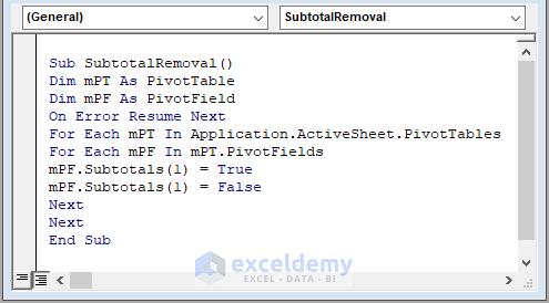

• Press F5.
• Return to the worksheet.

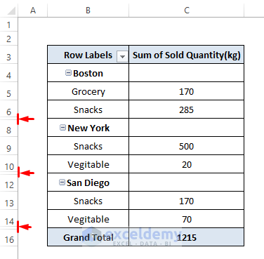
Method 5 – Hiding the Subtotal Rows in a Pivot Table

Steps:

• Place the cursor on City Subtotal’s Row Numbers and right-click on it.
• Select Hide from the Context Menu options.

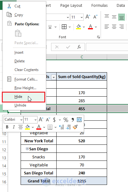
• Excel will remove the Subtotal Row (i.e., Row Number 7).

• Repeat for other Subtotal Rows and you see a final image similar to the following picture.

Read More: How to Subtotal Multiple Columns in Excel Pivot Table

Download the Excel Workbook

<< Go Back to Subtotals in Pivot Table | Pivot Table in Excel | Learn Excel