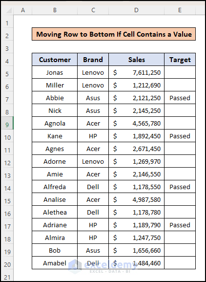
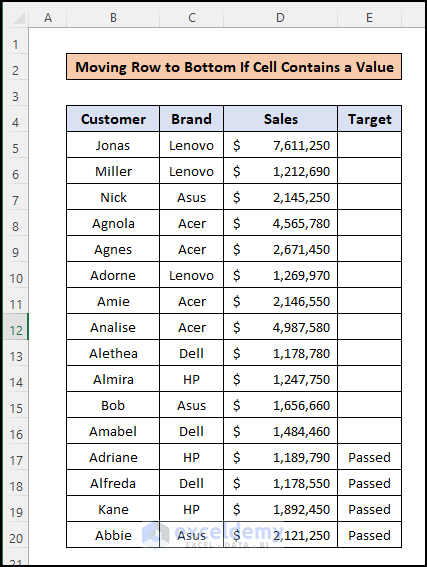
The sample dataset contains customer name, product brand name, sales amount, and target status. Some cells of the target column display “ Passed” . To move these rows to the bottom:
Method 1 – Move Row to Bottom If Cell Contains a Specific Text
Steps:
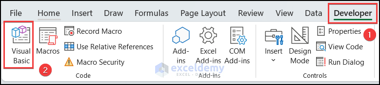
- Go to the Developer tab and click Visual Basic.
You can press ALT + F11 to open the Microsoft Visual Basic for Applications window.
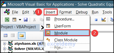
- Select “Insert” and choose “Module’”.
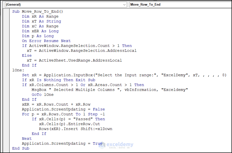
- Enter this VBA code:
Sub Move_Row_To_End()
Dim xR As Range
Dim xT As String
Dim xC As Range
Dim xER As Long
Dim p As Long
On Error Resume Next
If ActiveWindow.RangeSelection.Count > 1 Then
xT = ActiveWindow.RangeSelection.AddressLocal
Else
xT = ActiveSheet.UsedRange.AddressLocal
End If
lOne:
Set xR = Application.InputBox("Select the Input range:", "ExcelDemy", xT, , , , , 8)
If xR Is Nothing Then Exit Sub
If xR.Columns.Count > 1 Or xR.Areas.Count > 1 Then
MsgBox " Selected Multiple Columns ", vbInformation, "Exceldemy"
GoTo lOne
End If
xER = xR.Rows.Count + xR.Row
Application.ScreenUpdating = False
For p = xR.Rows.Count To 1 Step -1
If xR.Cells(p) = "Passed" Then
xR.Cells(p).EntireRow.Cut
Rows(xER).Insert Shift:=xlDown
End If
Next
Application.ScreenUpdating = True
End Sub
VBA Code Breakdown:
Segment 1:
Sub Move_Row_To_End()
Dim xR As Range
Dim xT As String
Dim xC As Range
Dim xER As Long
Dim p As Long
On Error Resume Next
The Move_Row_To_End new sub is created. 4 variables are declared and commanded to move to the next line if an error is found.
Segment 2:
If ActiveWindow.RangeSelection.Count > 1 Then
xT = ActiveWindow.RangeSelection.AddressLocal
Else
xT = ActiveSheet.UsedRange.AddressLocal
End If
If the number of selected cells is greater than 1, the selected range will be the input range of the code. Otherwise, it will select all used cells as the input range.
Segment 3:
lOne:
Set xR = Application.InputBox("Select the Input range:", "ExcelDemy", xT, , , , , 8)
This line creates an input box: “Exceldemy” to take the input of the cell range.
Segment 4:
If xR.Columns.Count > 1 Or xR.Areas.Count > 1 Then
MsgBox " Selected Multiple Columns ", vbInformation, "Exceldemy"
GoTo lOne
End If
If you select more than one column, a message box will display “Selected Multiple Columns”.
Segment 5:
xER = xR.Rows.Count + xR.Row
Application.ScreenUpdating = False
For p = xR.Rows.Count To 1 Step -1
If xR.Cells(p) = "Passed" Then
xR.Cells(p).EntireRow.Cut
Rows(xER).Insert Shift:=xlDown
End If
Next
Application.ScreenUpdating = True
End Sub
A For loop selects the rows containing the “Passed”, cut the row and paste it at the bottom of the sheet. The sub ends.
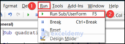
- Click Run and select the Run Sub/UserForm or press F5 to run the code.
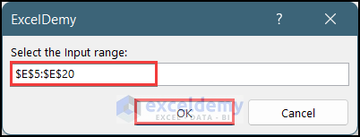
- In the pop-up window, enter the input range. Here, E5:E20.
- Click OK.
Rows containing “Passed” are at the bottom of the dataset.
Method 2 – Move a Row to Bottom If a Cell Contains a Number Greater Than a specified Number
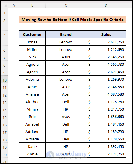
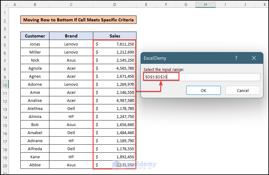
To move rows that contain sales values greater than $4,000,000 to the bottom of the dataset:
Steps:
- Open the dataset below in a new worksheet.
- Insert a new module:
- Enter this VBA code:
Sub Move_Row_To_End()
Dim xR As Range
Dim xT As String
Dim xC As Range
Dim xER As Long
Dim p As Long
On Error Resume Next
If ActiveWindow.RangeSelection.Count > 1 Then
xT = ActiveWindow.RangeSelection.AddressLocal
Else
xT = ActiveSheet.UsedRange.AddressLocal
End If
lOne:
Set xR = Application.InputBox("Select the Input range:", "ExcelDemy", xT, , , , , 8)
If xR Is Nothing Then Exit Sub
If xR.Columns.Count > 1 Or xR.Areas.Count > 1 Then
MsgBox " Selected Multiple Columns ", vbInformation, "Exceldemy"
GoTo lOne
End If
xER = xR.Rows.Count + xR.Row
Application.ScreenUpdating = False
For p = xR.Rows.Count To 1 Step -1
If xR.Cells(p) > 4000000 Then
xR.Cells(p).EntireRow.Cut
Rows(xER).Insert Shift:=xlDown
End If
Next
Application.ScreenUpdating = True
End Sub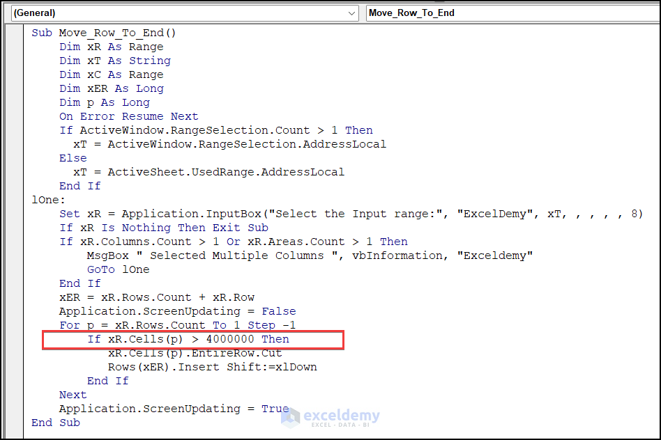
- Click Run.
- In the pop-up window, enter the input range. Here, D5:D20.
- Click OK.
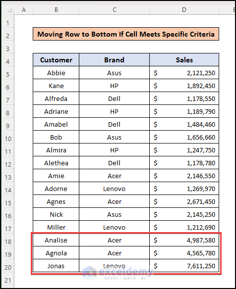
Rows containing sales greater than $4,000,000 are at the bottom of the dataset.
Read More: How to Move Row to Another Sheet Based on Cell Value in Excel
Download Practice Workbook
Download the practice workbook.
Related Articles
- How to Move Rows Down in Excel
- How to Move Rows in Excel to Columns
- How to Move Every Other Row to Column in Excel
- How to Move Rows Up in Excel
- How to Move Rows in Excel Without Replacing
- How to Rearrange Rows in Excel
<< Go Back to Move Rows | Rows in Excel | Learn Excel
Get FREE Advanced Excel Exercises with Solutions!
