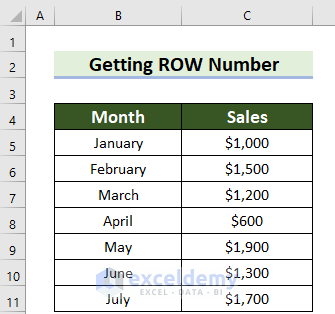
In this article we will cover four methods of how to get the Row Number of a Current cell in Excel. The sample dataset contains two columns. These are Month and Sales.
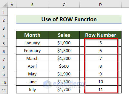
Method 1 – Use the ROW Function to Get Row Number
The ROW function is a built-in function in Excel.
Steps:
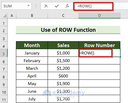
- Select a cell (D5 here) where you want to keep the Row Number. The selected cell should be horizontally adjacent to the relevant row.
- Enter the formula in the D5 cell.
=ROW()
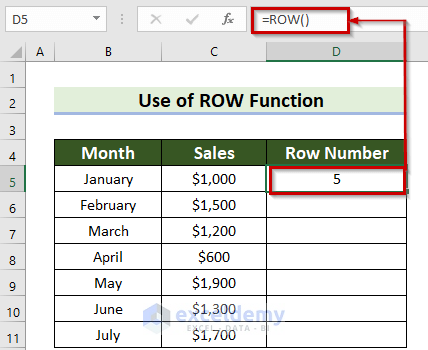
- Press ENTER to get the Row Number.
- Drag the Fill Handle icon to AutoFill the corresponding data in the rest of the cells D6:D11.
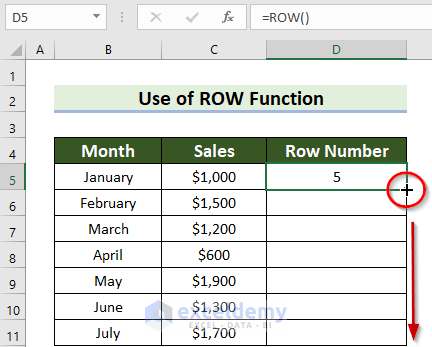
- All the corresponding Row numbers will be returned.
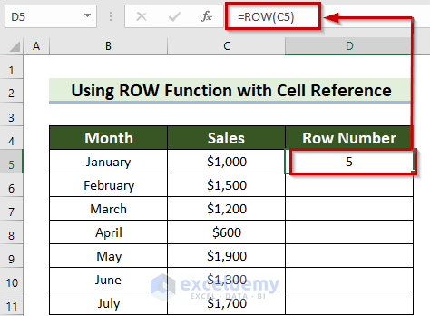
Method 2 – Employing ROW Function with a Cell Reference to Get Row Number of Current Cell
Here, we use the ROW function with a cell reference to get the Row Number of a cell in Excel.
Steps:
- Select a cell (D5 in this instance) where the Row Number should be entered.
- The selected cell should be horizontally adjacent to the relevant row.
=ROW(C5)The ROW function will return the Row number of the reference cell. Here, C5 is the reference.
- Press ENTER to get the Row Number.
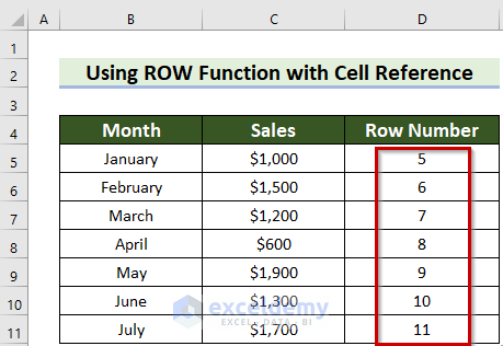
- Double-click on the Fill Handle icon to AutoFill the corresponding data in the rest of the cells D6:D11.
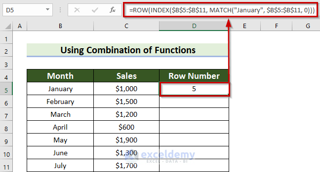
Method 3 – Combining Functions to Get the Row Number of Current Cell
In this method the ROW, INDEX, and MATCH functions are used in combination to get the Row number of the Current cell.
Steps:
- Select a cell where you want to keep the Row Number.
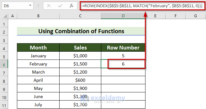
- Use the following formula in the D5 cell.
=ROW(INDEX($B$5:$B$11, MATCH("January", $B$5:$B$11, 0)))- Press ENTER to get the Row Number.
Formula Breakdown
- The MATCH function will return the relative position of a cell value in a given array.
- The Array is $B$5:$B$11. The Dollar ($) sign denotes that the array is fixed.
- MATCH(“January”, $B$5:$B$11, 0)—> becomes 1.
- The INDEX function will return the cell value from a given array using a specified position.
- INDEX($B$5:$B$11, 1)—> turns January.
- The ROW function will take January as reference.
- Output: 5.
- To find the Row number of another cell value, insert that cell value inside Inverted Commas.
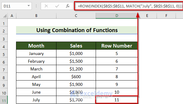
- Use the below formula in cell D6.
=ROW(INDEX($B$5:$B$11, MATCH("February", $B$5:$B$11, 0)))- Then, press ENTER to get the Row Number.
Do the same for the other cell values.
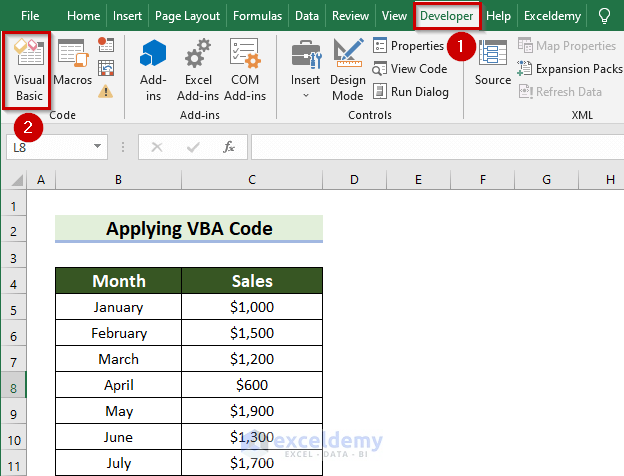
Method 4 – Applying VBA to Get Row Number of Current Cell in Excel
You can employ VBA code to get the Row Number of a cell.
Steps:
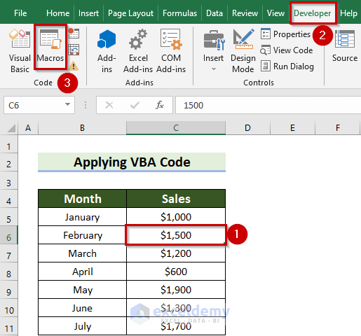
- From the Developer tab >> choose the Visual Basic command.
The Excel file must be saved as an Excel Macro-Enabled Workbook (*xlsm).
- From the Insert tab >> select Module.
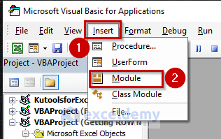
- Enter the following code in the Module1.
Sub Row_No_of_Current_Cell()
Dim my_Row_No As String
my_Row_No = ActiveCell.Row
MsgBox my_Row_No
End Sub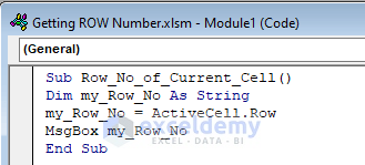
Code Breakdown
- Here a Sub Procedure named Row_No_of_Current_Cell has been created.
- The variable my_Row_No is used as a String.
- Row is used to count the Row number.
- MsgBox will show the result.
- Save the code.
- Go to the Excel worksheet.
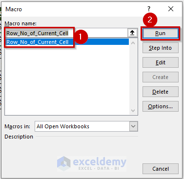
- Select the cell for which you want to get the Row number.
- From the Developer tab choose Macros.
- Select Row_No_of_Current_Cell from the Macro name.
- Click Run.
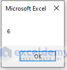
A dialog box named Microsoft Excel will appear with the corresponding Row number.
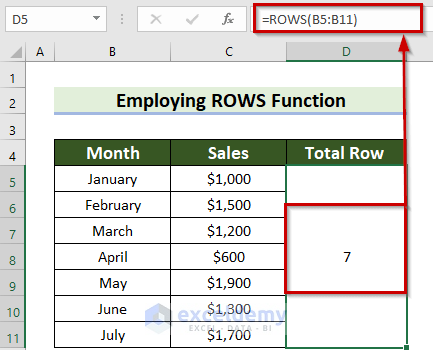
Use of ROWS Function to Get Number of Rows in a Range of Cells
There is another function in Excel to count the Total Rows number inside a given array.
Steps:
- Select a cell where you want to enter the Total Row Numbers. Here, the cells D5:D11 are selected.
- Enter the formula in the D5:D11 cells.
=ROWS(B5:B11)The ROWS function will return the Total Row numbers of the given array, which is B5:B11 in this example.
- Press ENTER to get the Row Number.
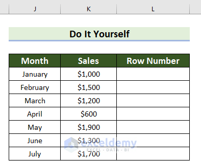
Practice Section
Now, you can practice by yourself.
Download Practice Workbook
You can download the practice workbook from here:
Related Articles
- Find String in Column and Return Row Number in Excel
- How to Use Range with Variable Row Number in Excel
<< Go Back to Rows in Excel | Learn Excel
Get FREE Advanced Excel Exercises with Solutions!
