How to Use DSUM Function with Dynamic Criteria in Excel

Excel’s DSUM function is used to extract and sum a set of data from a database. It computes the sum of a set of data that meets certain criteria. In this article, we will discuss how to use the DSUM function with dynamic criteria in Excel.

The attached GIF given below is an overview of the discussion which depicts the output of the DSUM function with dynamic criteria in Excel.

Download Practice Workbook

You can download and practice the dataset that we have used to prepare this article.

2 Practical Examples to Use DSUM Function with Dynamic Criteria in Excel

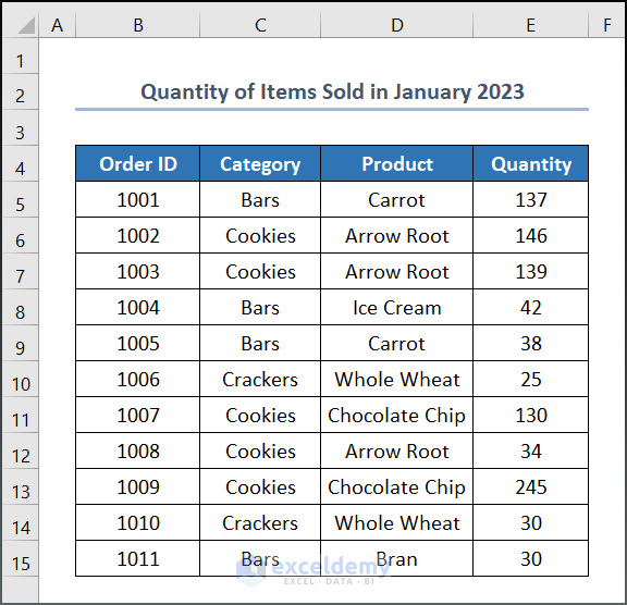
Let’s assume we have a dataset, namely “Quantity of Items Sold in January 2023”. You can use any dataset suitable for you.

Here, we have used the Microsoft Excel 365 version; you may use any other version according to your convenience.

Example 1: Use of DSUM Function with Dynamic Single Criteria

The basic outline of the DSUM function can be written as =DSUM(database, field, criteria). Where the argument criteria may be single or multiple. In our first example, we will talk about dynamic single and its uses.

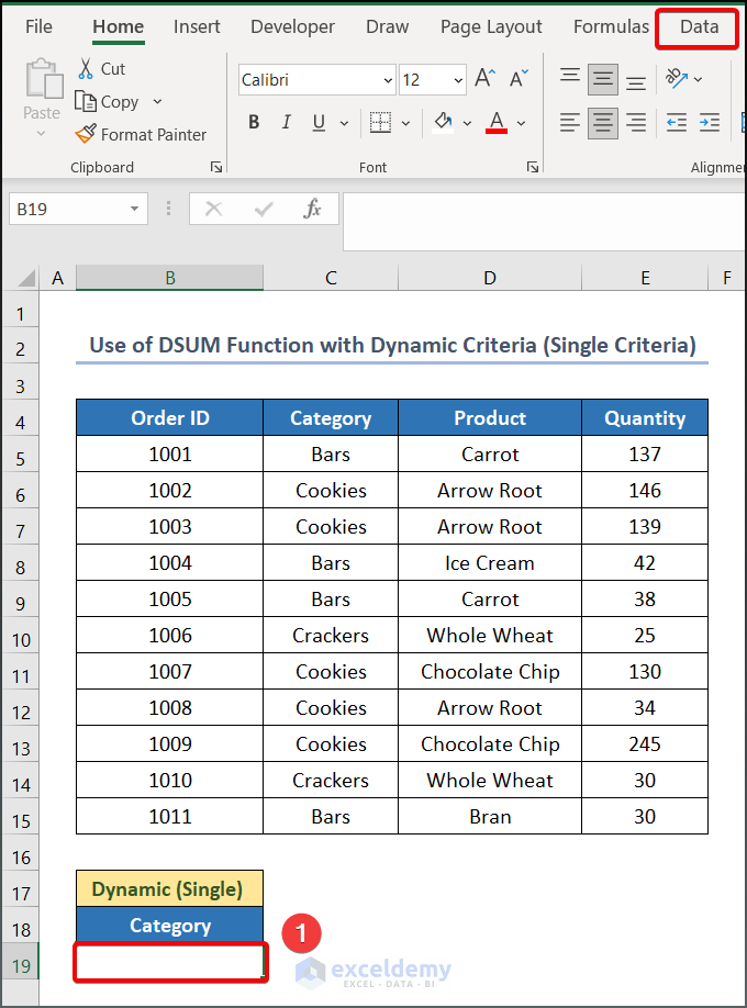
Step 1: Set Dynamic List using Data Validation Feature

In our first step, we will discuss how to use the Data Validation feature to build a dynamic drop-down list. Using an Excel drop-down list, data is entered into a spreadsheet from a pre-defined list of items. Thus, it enables users to submit data more quickly and precisely than doing it manually.

• To proceed with this process, select cell B19.
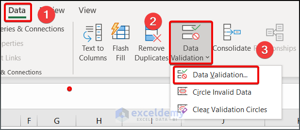
• Move on to the Data tab of the Menu Bar.

• Select Data > Data Validation from Excel Ribbon.

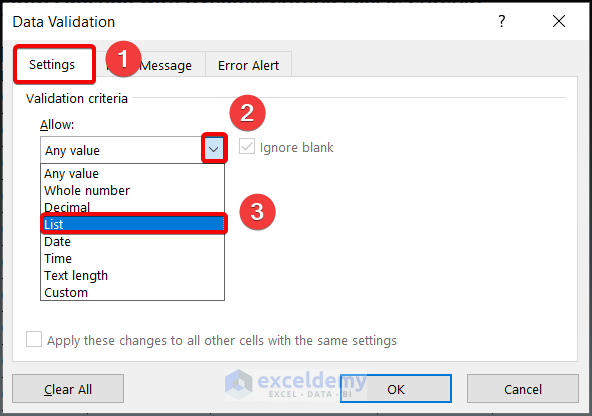
• Subsequently, a dialog box will appear. Now select the Settings tab then choose List from the drop-down options of Allow.

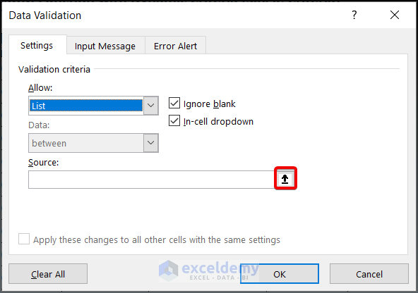
• Thus, an additional box will appear named Source in the dialog box.
• Click on the Upwards arrow.

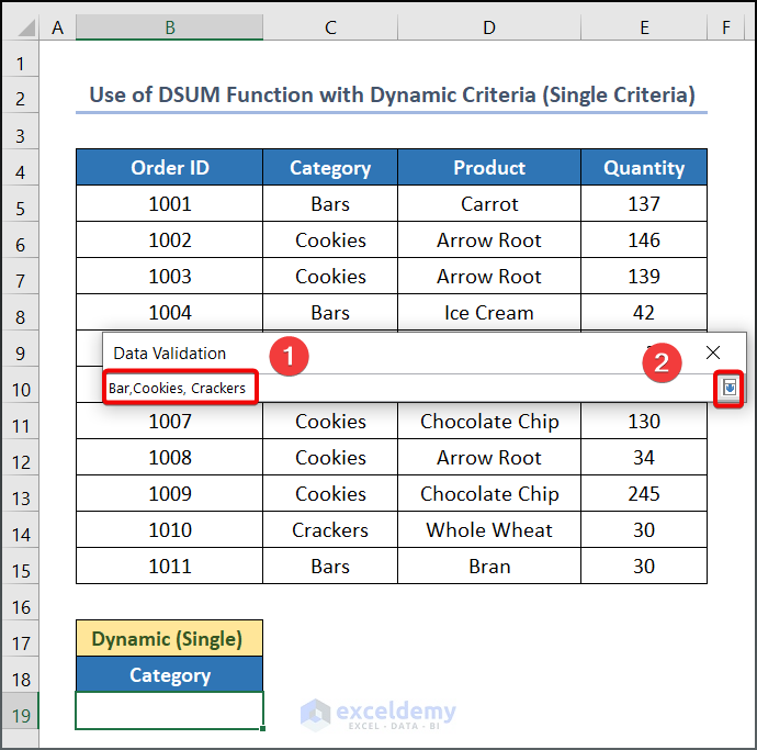
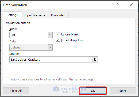
• Now type your drop-down list data in this box. For this specific dataset, we input Bar, Cookies, Crackers as only those items exist in a repetitive manner under the Category column.
• Subsequently, click on the Downwards arrow to close the dialog box.

• Press OK afterward.

Step 2: Use of DSUM Function on Dynamic List

As our dynamic drop-down list is ready, we will now plug the dynamic drop-down list as criteria into the DSUM function. Follow the process we are going to describe below.

• Write the following formula in cell D19.

This action will allow us to have the output. However, before going to show you the result, let’s put some paint on the cell to make our criteria more discernible.

• From the Menu Bar, select Home > Conditional Formatting > Highlights Cells Rules >Text That Contains…

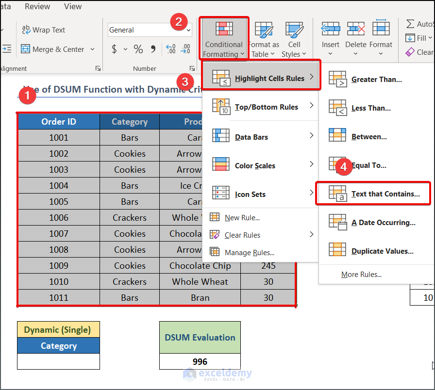
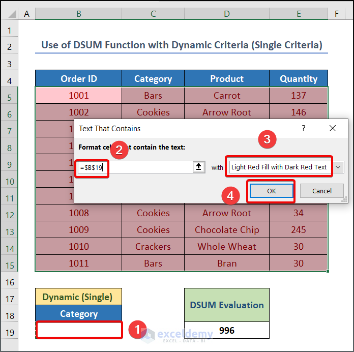
• Subsequently, a dialogue box will pop up.
• Select the B19 cell, then click on Light Red Fill with Dark Red Text. Though you can also select any of the options in with box according to your preference.
• Press on OK

• Now see the output as given in the attached GIF.

Read More: Excel DSUM vs SUMIF Functions (2 Suitable Examples)

Similar Readings

• How to Use Excel DMAX Function (2 Easy Examples)
• Calculate Standard Deviation with IF Conditions in Excel
• How to Use Macaulay Duration Formula in Excel (2 Easy Methods)
• Determine If a Number Is Even in Excel (4 Suitable Ways)
• How to Use DOLLAR Function in Excel (5 Suitable Examples)

Example 2: Use of DSUM Function with Dynamic Multiple Criteria

In our first example, we selected one cell as our argument, which was labeled as single-column dynamic criteria; however, in the second example, we will work on dynamic multiple criteria.

The process will be the same as what we did in the first example. All you have to add an extra drop-down list based on the list of items under the Product header.

Step 1: Create Dynamic List using Data Validation Feature

• Create another drop-down list by using the Data Validation feature and have the output as given below.

Step 2: Employ the DSUM Function on Dynamic List

• Now write the following formula in cell E19.

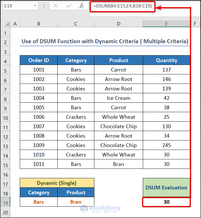
• After filling the cell with the Conditional Formatting feature, you will have an output as given below.

Read More: How to Use DSUM Function with Multiple Criteria in Excel

Things to Remember

• It is important to select the Header while selecting the range of data as your Database and Criteria. Otherwise, you will not get any output.

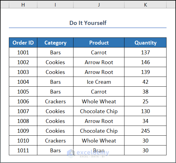
Practice Section

We have provided a Practice section on the right side of each sheet, so you can practice yourself. Please make sure to do it yourself.

Conclusion

In this article, we have discussed how to use DSUM function with dynamic criteria in Excel. The use of this function may vary with your dataset. So before going through a specific way, ensure the method you choose aligns with your work. Further, If you have any queries, feel free to comment below and we will get back to you soon.

Related Articles

• How to Use DVAR Function in Excel (2 Suitable Examples)
• [Fixed!] EDATE Function Not Working in Excel
• How to Use DCOUNT Function in Excel (5 Suitable Examples)
• Use DSTDEV Function in Excel (3 Practical Examples)
• How to Use DMIN Function in Excel (4 Suitable Examples)
• Can Excel DGET Return Multiple Records [See 4 Solutions]
• How to Use Database Functions in Excel (With Examples)