How to Consolidate Data from Multiple Workbooks in a Single Worksheet (3 Examples)

Method 1 – Consolidate Data of Similar Tables from Multiple Workbooks

Steps:

• Consolidate 4 Excel files.

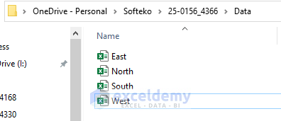
• We have a table named Profit in our dataset.

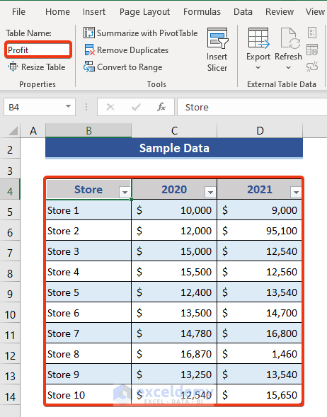
Each of the 4 Excel files has tables of the same name and format.

• Apply the Power Query.
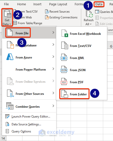
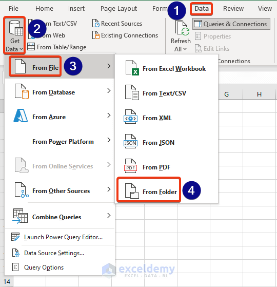
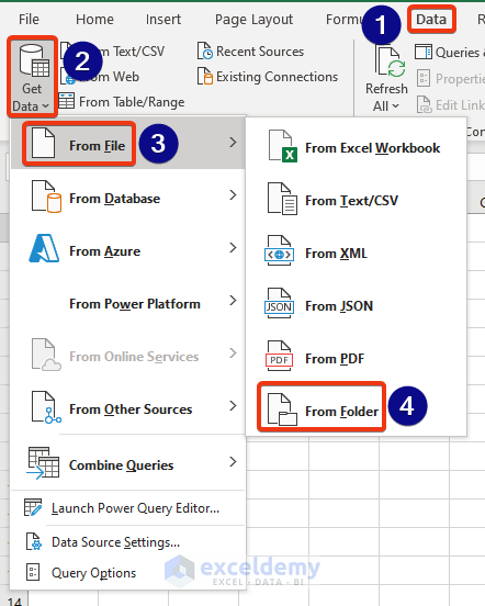
• Click on the Data tab.
• Choose From File of the Get Data option.
• Choose the From Folder option.

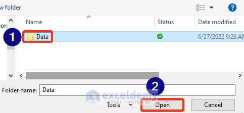
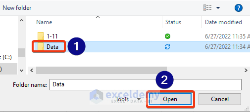
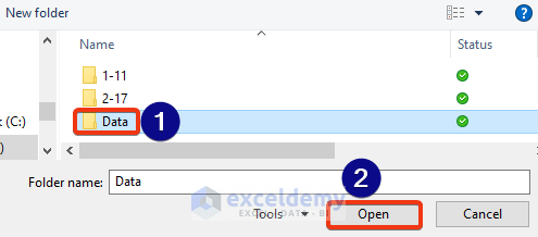
• Select the Data folder from the File Explorer.
• Press the Open button.

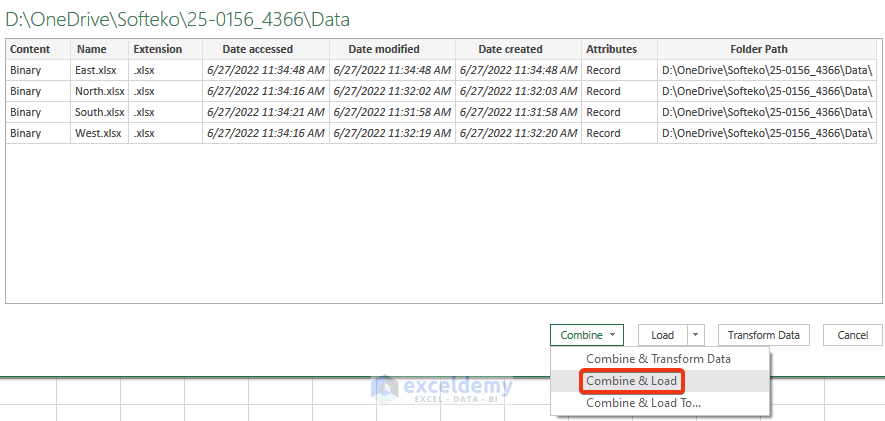
• A window appears showing the file details.

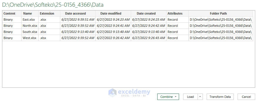
Click on the image for better quality

• Press the Combine & Load button.

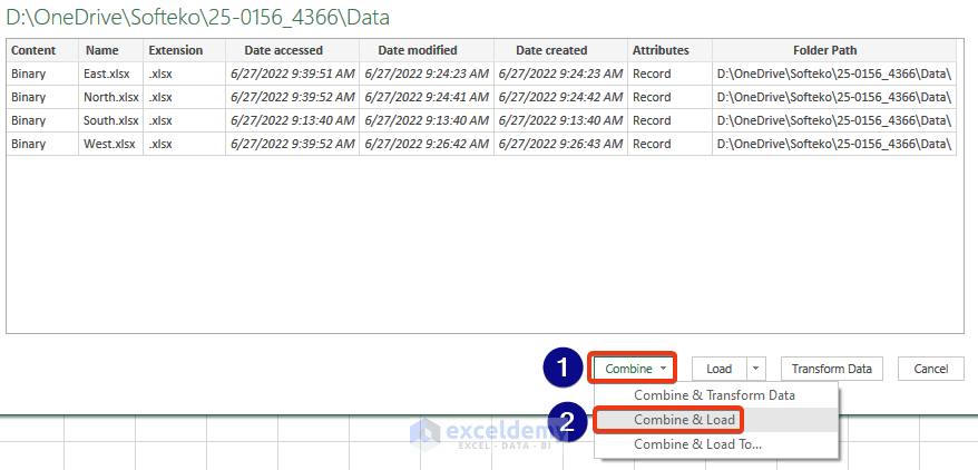
Click on the image for better quality

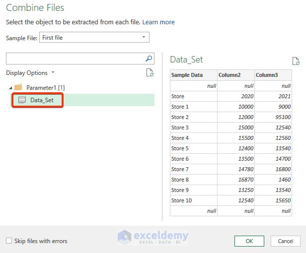
• Select the Profit table and press OK.

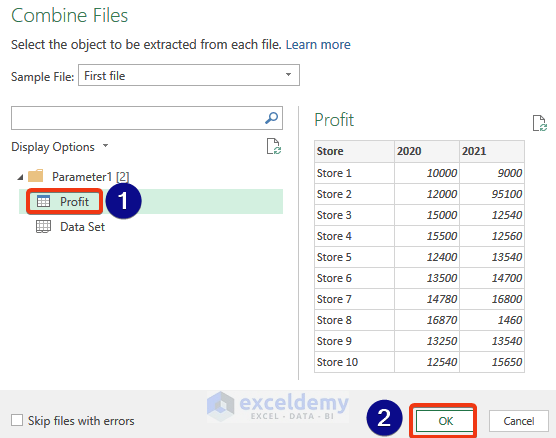
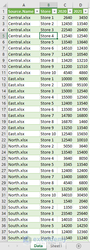
All data is combined from multiple workbooks into a single sheet.

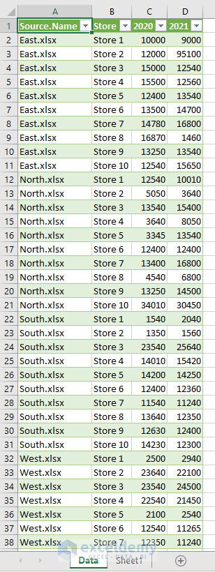
Click on the image for better quality

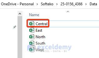
If we want to add more files to the dataset, add a file in the same folder in the same format.

• We added a new file named Central.

• Go to any cell of the combined file. Right-click
• Choose the Refresh button option from the Context Menu.

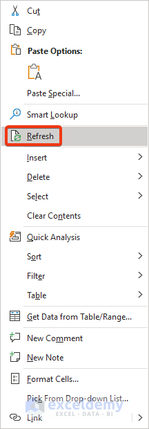
Have a look at the dataset.

Click on the image for better quality

Method 2 – Merge Data from Multiple Workbooks with the Same Worksheet Names

Steps:

• See the Sheet Name at the bottom section.

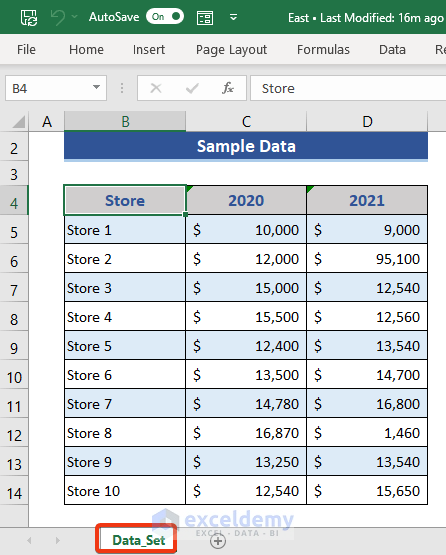
All the workbooks consist of worksheets of the same name.

• Click on the Data tab.
• Follow Get Data >> From File >> From Folder.

• Select the desired folder from the File Explorer.
• Press Open.

• A window appears with the file name and details.
• Click on the Combine & Load option.

Click on the image for better quality

• Choose the Sheet name from the Combine file window.

If we have other sheets in the workbooks, those will also show here.

• Press OK.

Click on the image for better quality

Data from multiple workbooks with the same-named worksheets are combined here.

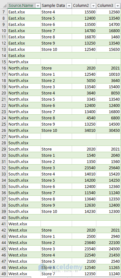
Method 3 – Consolidate Multiple Workbooks with Different Table and Sheet Names

Steps:

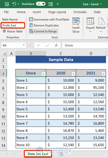
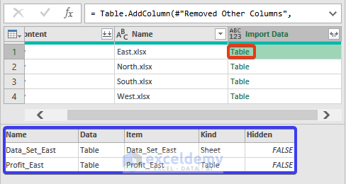
Below is the table and sheet name of the East file.

Here is the West file.

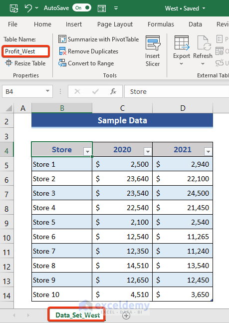
Table and Sheet Names are different for both cases.

• Click on the Data tab.
• Go Get Data >> From File >> From Folder.

• Choose the desired file from the File Explorer.
• Press the Open button.

• The file with details is shown here.
• Click on the Transform Data button in the window.

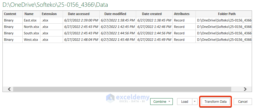
Click on the image for better quality

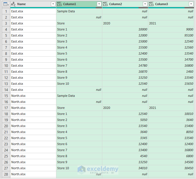
• Enter the Power query mode.

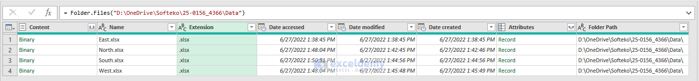
Click on the image for better quality

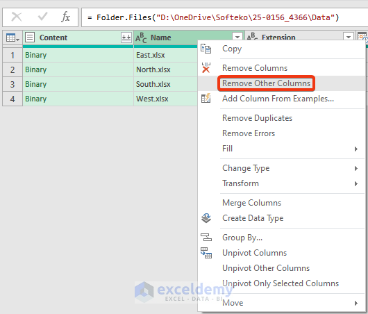
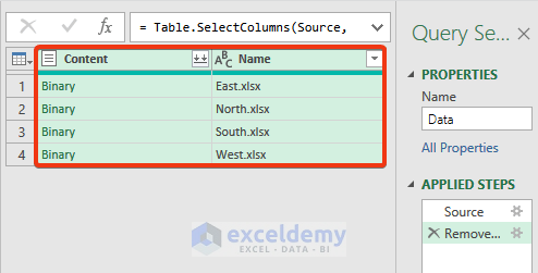
We do not need to appear in all the columns here.

• Choose the Content and Name column and right-click.
• Choose the Remove Other Columns option.

• Two columns are shown here.

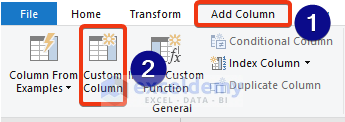
• Press the Add Column tab.
• Select the Custom Column option.

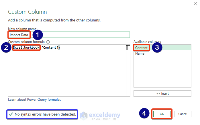
• The Custom Column window will appear.
• Insert the name Import Data from the new column.
• We need to use a formula here. The exact formula is here. Click on the Content option.

• After entering the formula, a green check mark will show that no errors are available to her.
• Press OK.

• We can see a new column added here.

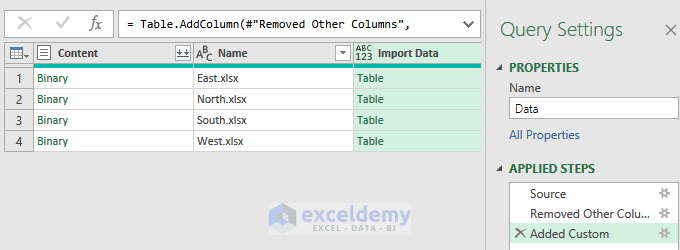
• Click on any cell of the Import Data details shown here.

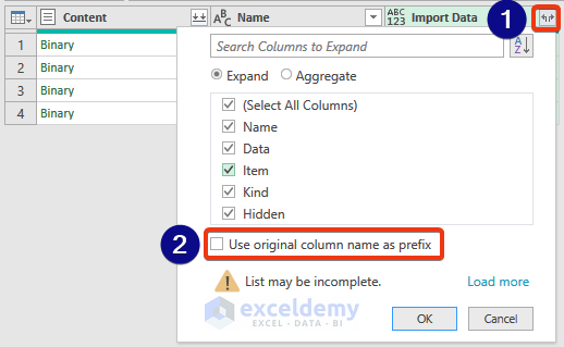
• Expand the Import data column.
• Click on the right-upper side of the Import Data column.
• A menu shows to check options. We uncheck the Use original column name as the prefix.
• Press the OK button.

• Data has expanded.

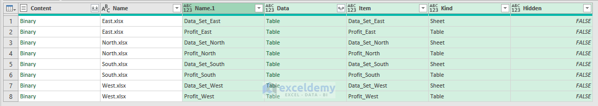
Click on the image for better quality

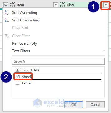
• Both Sheets and Tables are shown. But we want only sheets and tables will be included in the Sheets.
• Click the arrow in the Kind column.
• Check only the Sheet option.
• Press OK.

• We do not need all the rows here.

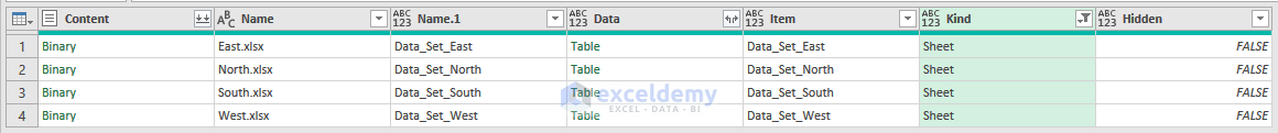
Click on the image for better quality

• Choose the Name and Data columns and press the right button on the mouse.
• Click on the Remove Other Columns option.

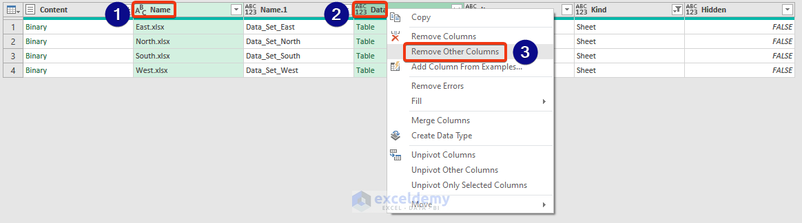
Click on the image for better quality

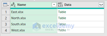
• We can see the two columns.

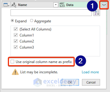
• Click on the right-upper corner of the Data column.
• Uncheck the use of the original column name as the prefix.
• Press OK.

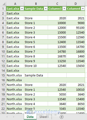
• We get all the data.

• Click on the Transform tab.
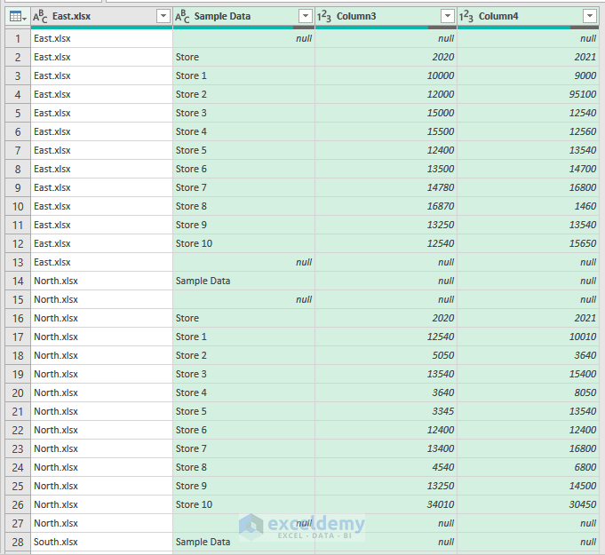
• Choose the Use First Row as Headers option.

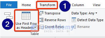
• The header has changed now.

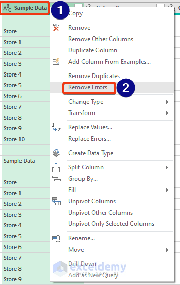
• We want to remove the errors. Press the right button of the mouse. Click on the Remove Errors from the Context Menu.

• Go to the Home tab.
• Click on the Close & Load option.

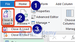
• We get our data.

Download the Practice Workbooks

Download this workbook to practice.