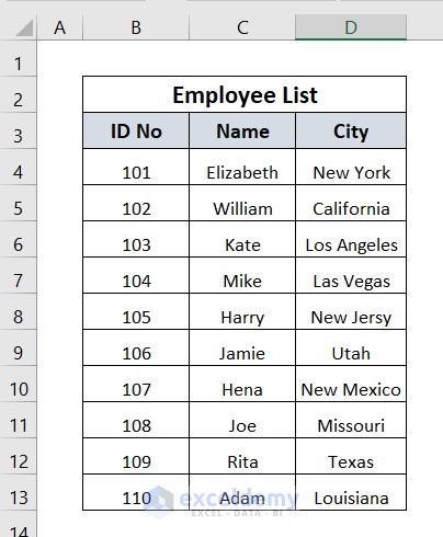
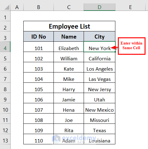
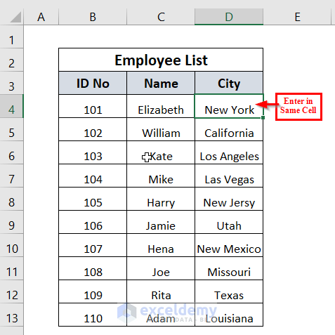
The following Employee List table shows ID No, Name, and City columns. Using this table, we will show you how to enter within the cell.
Method 1 – Using Keyboard Shortcut to Enter within a Cell
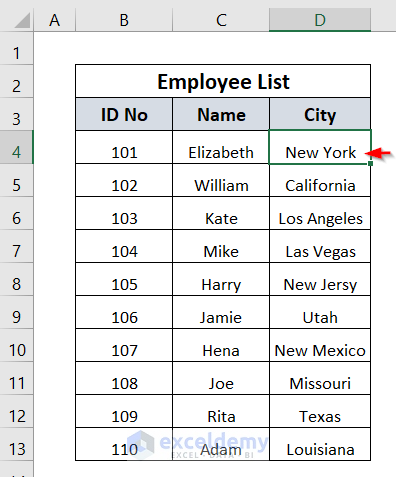
Click on cell D4.
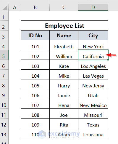
However, after we press Enter, we automatically move to the down cell D5.
- To remain in the same cell D4, first of all, we have to type Ctrl+Enter.
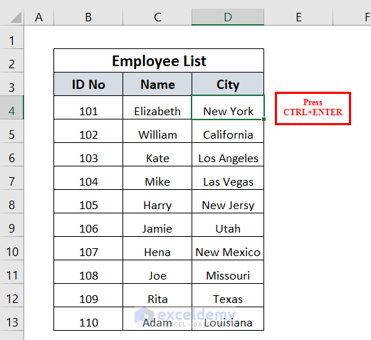
- Now, if we press Enter, we stay in the same cell D4.
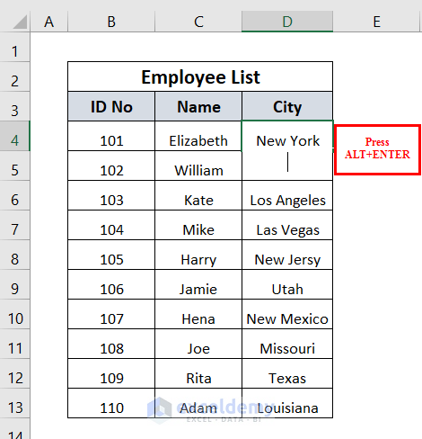
Let’s create a line in the same cell:
- Type Alt+Enter in our cell D4.
We can see a new line is created in the same cell.
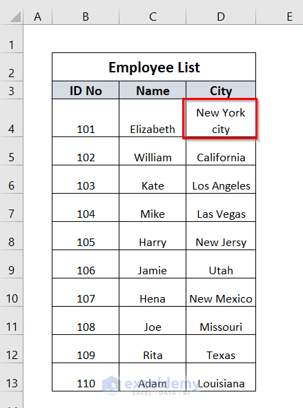
- Type anything in cell D4, and press Enter. We can see two lines of data in cell D4.
Read More: How to Add New Line with CONCATENATE Formula in Excel
Method 2- Stay in Same Cell after Pressing ENTER with Excel Options
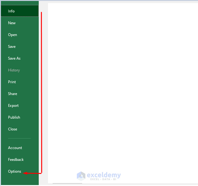
- Go to the File tab in the ribbon.
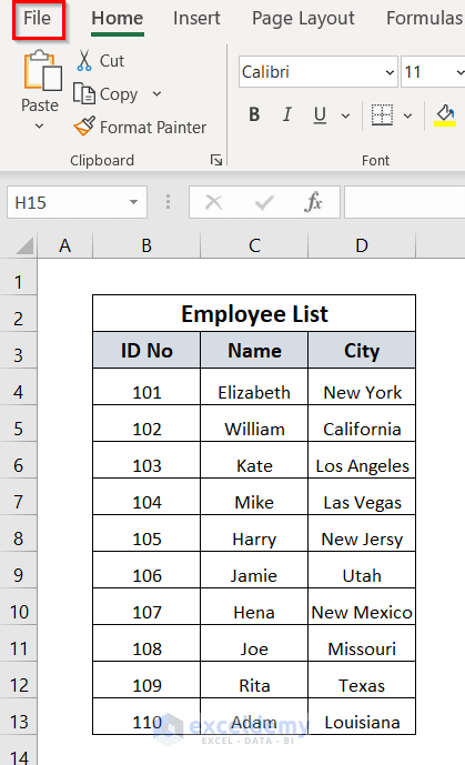
- Select Options.
An Excel Options window will appear.
- Select Advanced, unmark After pressing Enter move selection, and click OK.
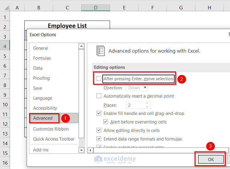
- We can see that even if we press ENTER in cell D4, we stay in the same cell D4.
Read More: Excel: Inserts New Line in Cell Formula
Method 3 – Using TEXTJOIN Function to Enter within a Cell
This method works for Office 365, Excel 2019, and Excel 2019 for Mac, and newer.
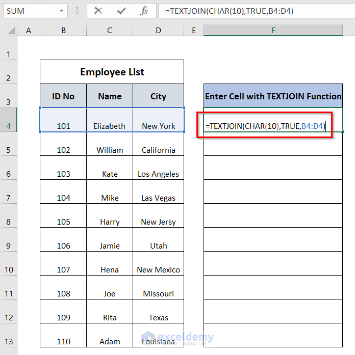
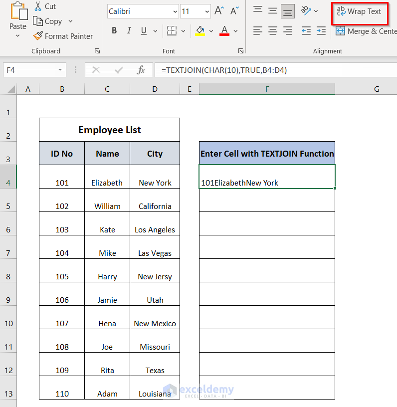
- Type the following function in cell F4.
=TEXTJOIN(CHAR(10),TRUE,B4:D4) Here, CHAR(10) → adds a carriage return between each combined text value.
TRUE → tells the formula to skip empty cells.
B4:D4 → are the cells to join.
- Press Enter.
We can see the result in cell F4.
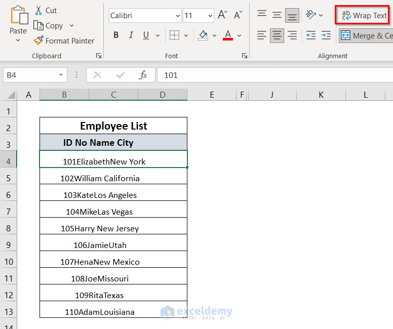
- Sellect F4 and click on Wrap Text.
Here, we can see 3 lines in one cell F4.
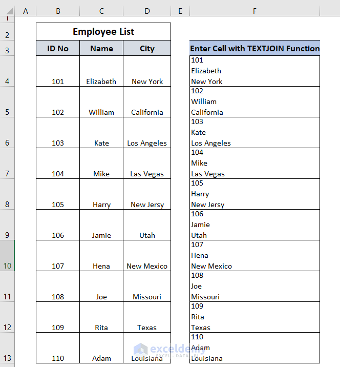
- Drag down the formula with the Fill Handle tool.
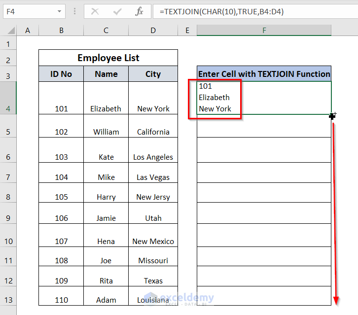
- All the cells from F4 to F13 contain 3 lines of information in one cell.
Read More: How to Put Multiple Lines in Excel Cell
Method 4 – Using CONCATENATE Function
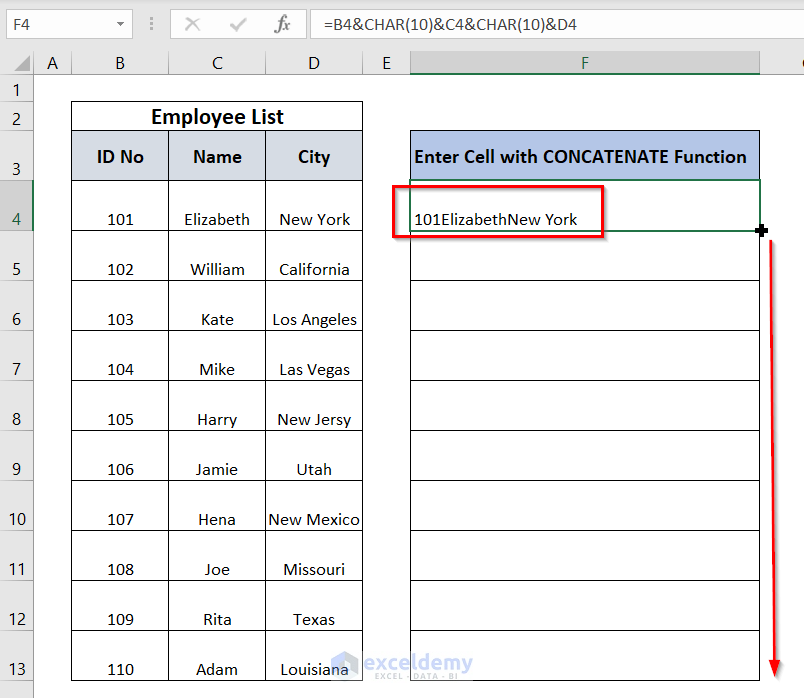
- Type the following formula in cell F4:
=B4&CHAR(10)&C4&CHAR(10)&D4Here, the CHAR function helps us to insert line breaks in between.
- Press ENTER.
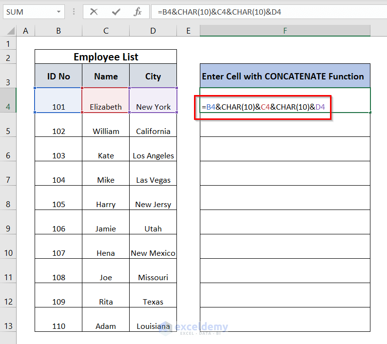
We can see the result in cell F4.
- Drag down the formula with the Fill Handle tool.
We can see that the information from multiple cells is now put together in a single cell.
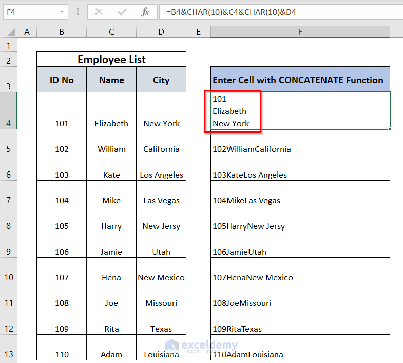
- Click on cell F4 and then click on Wrap Text.
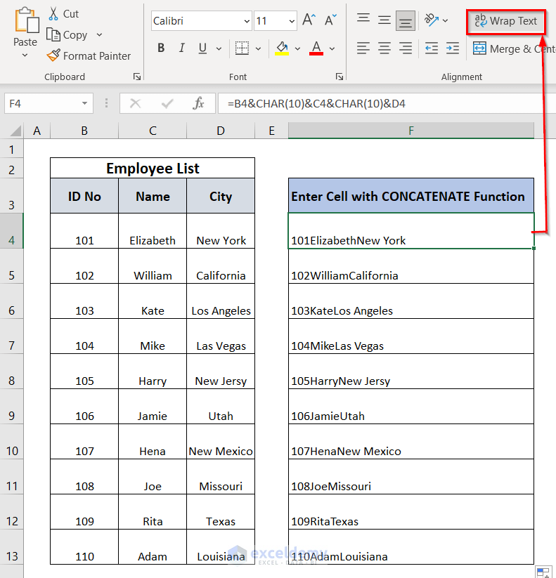
Finally, we can see the wrap text with three line breaks in cell F4.
Method 5 – Using Replace Option to Insert Line Break in a Cell
In this method, we want to remove commas from ID No, Name and City, and we want to insert line breaks instead.
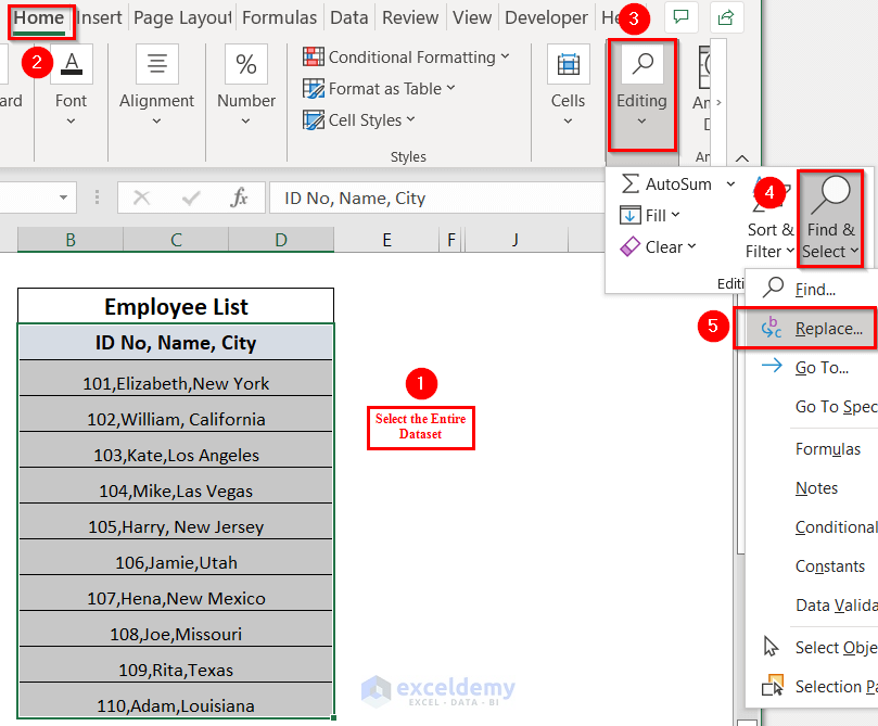
- Select the entire dataset of the table.
- Go to the Home tab, choose the Editing option, Find & Select option, and select Replace.
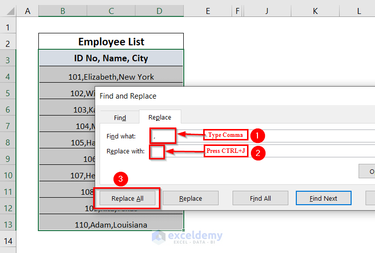
A Find and Replace window will appear.
- Type a comma ”,” in the Find what box.
- In the Replace with box, press CTRL+J.
- Select Replace All.
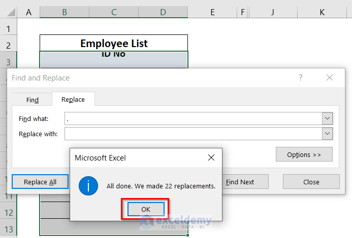
A Microsoft Excel window will appear.
- Click on OK.
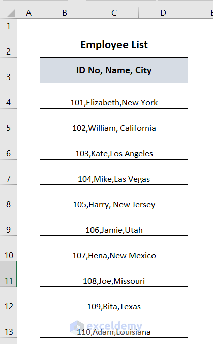
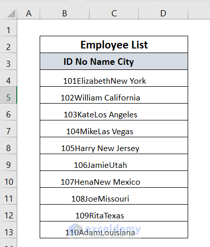
Finally, we can see there is no comma in the Employee List table.
To see line breaks in a cell between the ID No, Name, and City, we have to click on any of the cells.
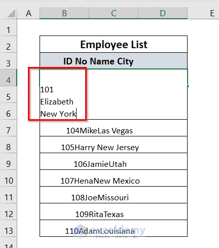
- We selected the merged cell B4:D4.
- Click on Wrap Text.
Finally, we can see three line breaks in the merged cell B4:D4.
You can do the same for the others following the process.
Download Workbook
Related Articles
<< Go Back to New Line | Text Formatting | Learn Excel
Get FREE Advanced Excel Exercises with Solutions!
