How to Draw Arrows in Excel – 3 Methods

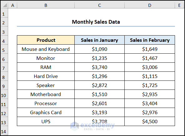
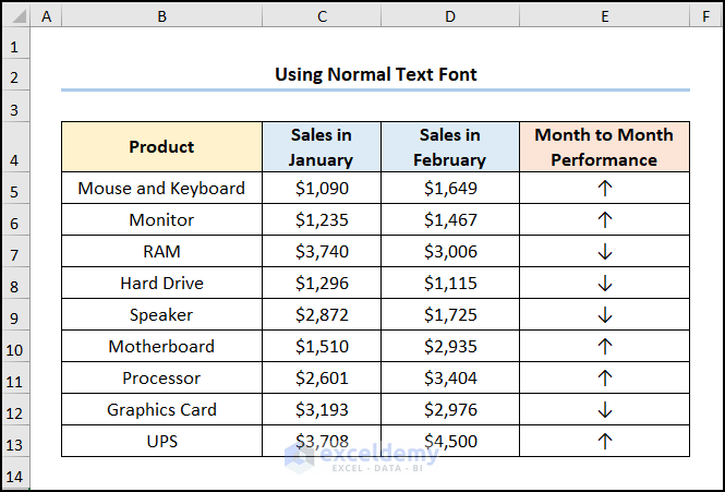
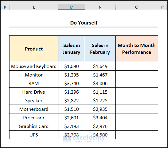
Consider the dataset below.

It showcases Product names and Sales in January and in February. Insert an up or a down arrow to indicate the increase or decrease in sales between the two months:

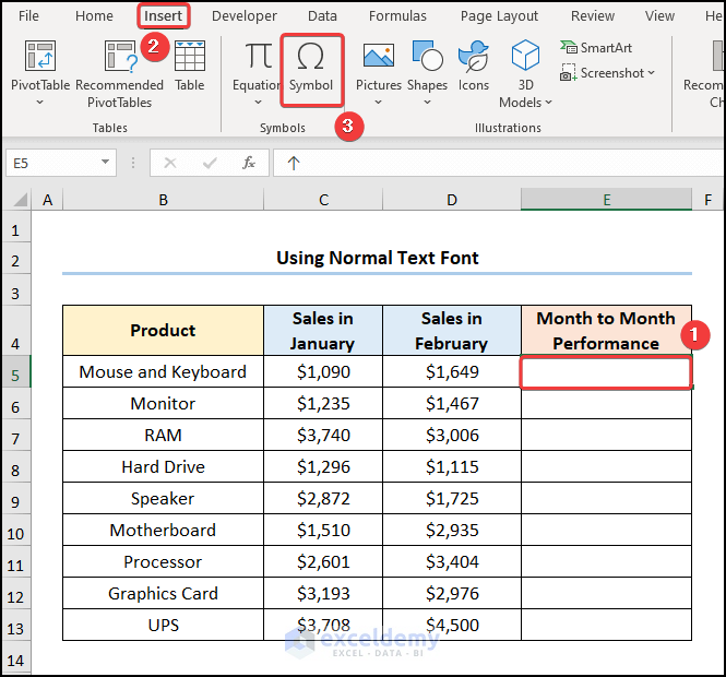
Method 1 – Draw Arrows Using Symbol Option

1.1 Using a Normal Text Font to Draw Arrows

Steps:

• Go to E5 >> click Insert >> select Symbol.

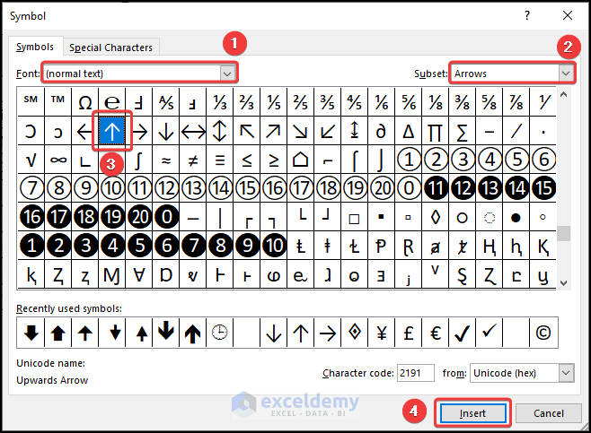
• In Font, choose (normal text).
• In Subset, select Arrows.
• Choose an arrow and click Insert.

This is the output.

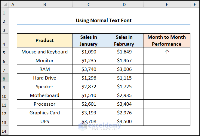
Repeat the procedure for the other cells:

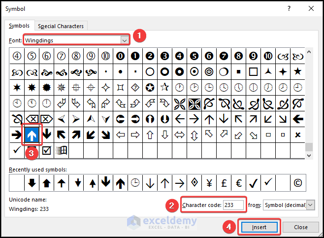
1.2 Using the Wingdings Font to Draw Arrows

Steps:

• Go to E5 >> click Insert >> select Symbol.

• Select Wingdings in Font >> enter 233 in the Character Code box.
• Select the arrow shown below >> click Insert.

This is the output.

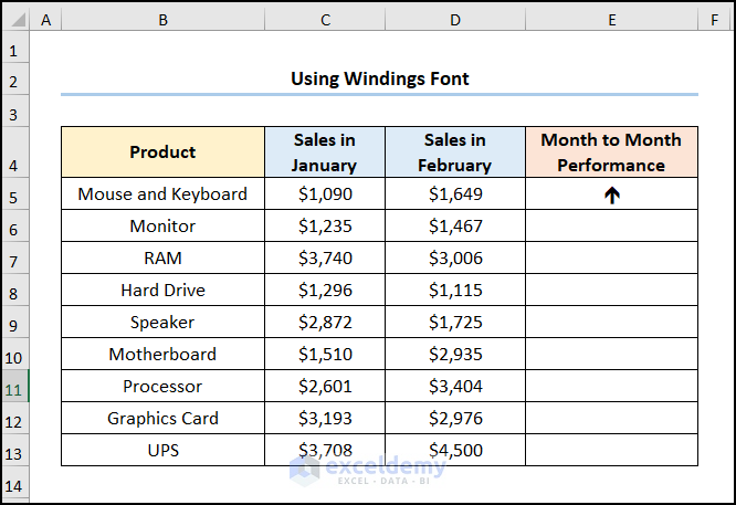
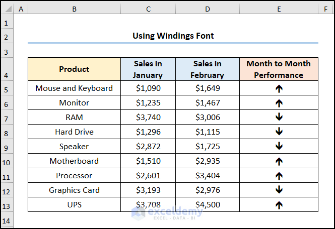
• Repeat the procedure for the other cells:

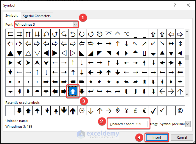
1.3 Using Wingdings 3 Font to Draw Arrows

Steps:

• Go to E5 >> click Insert >> select Symbol.

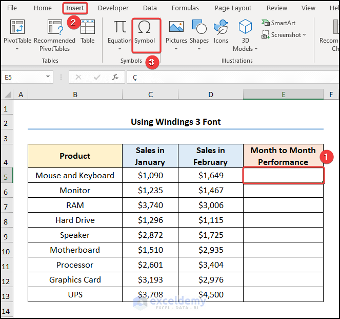
• Choose Wingdings 3 in Font >> enter 199 in Character Code and choose the arrow shown below >> click Insert.

• Repeat the procedure for the other cells:

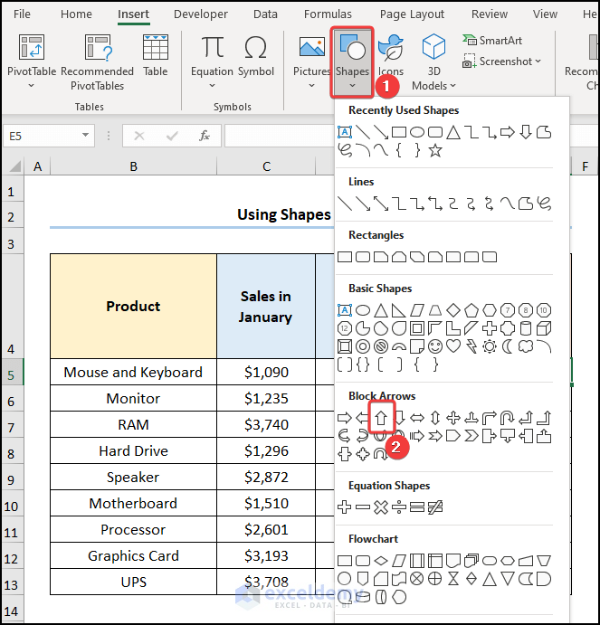
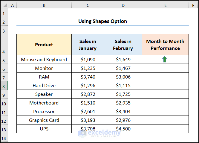
Method 2 – Using the Shapes Option to Draw Arrows

Steps:

• Go to E5 >> click Insert >> select Shapes.

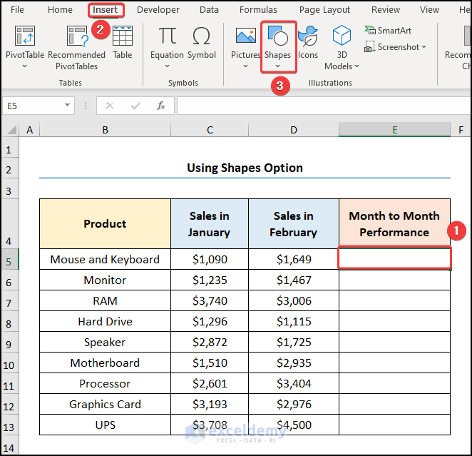
• In Block Arrows, choose the up arrow.

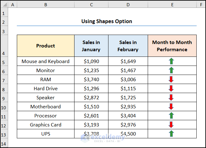
• Left-click and hold the mouse button, and drag the cursor to draw an arrow. You can move, resize, and change the color of the arrow.

• Insert a down arrow following the above procedure.
• Copy the arrows into their locations as shown below.

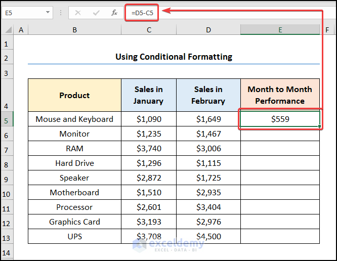
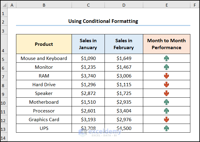
Method 3 – Applying Conditional Formatting to Draw Arrows

Steps:

• Go to the E5 and enter the expression below.

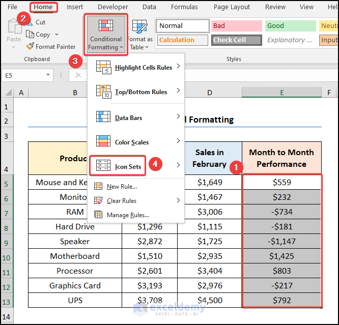
• Select E5:E13>> click Conditional Formatting >> choose Icon Sets.

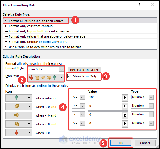
In the New Formatting Rule dialog box:

• Choose Format cells based on their values.
• In Format Style, choose Icon Sets and check Show Icon Only.
• Enter a value. Here, 100.

This is the output.

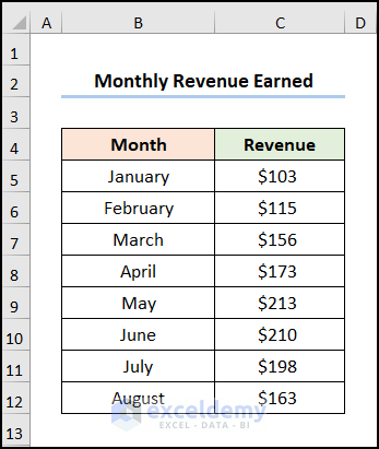
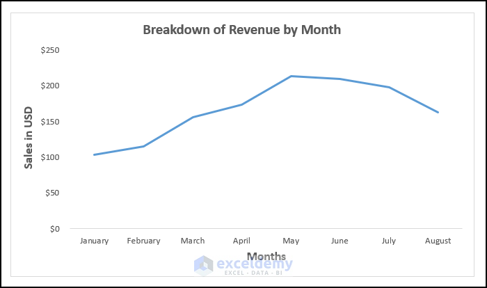
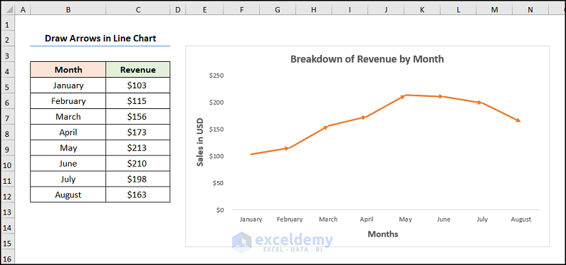
Draw Arrows in a Line Chart

Consider the dataset below. It showcases a breakdown of the Revenue from January to August.

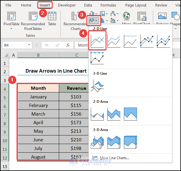
Steps:

• Select B4:C12 >> go to the Insert tab >> in Charts, click Insert Line or Area Chart >> choose Line.

You can also format the chart using the Chart Elements:

• Enable the Axes Title and enter the axis name. Here, Breakdown of Revenue by Month.
• Add a Chart Title. Here, Month and Sales in USD.
• Uncheck Gridlines.

This is the output.

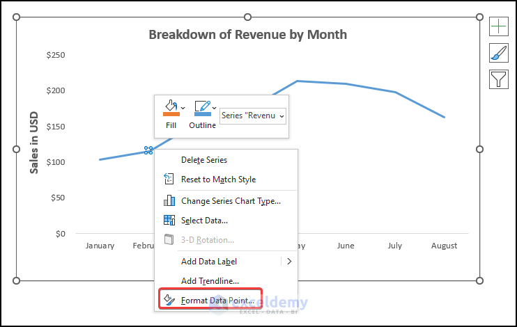
• Select a data point and right-click to go to Format Data Point.

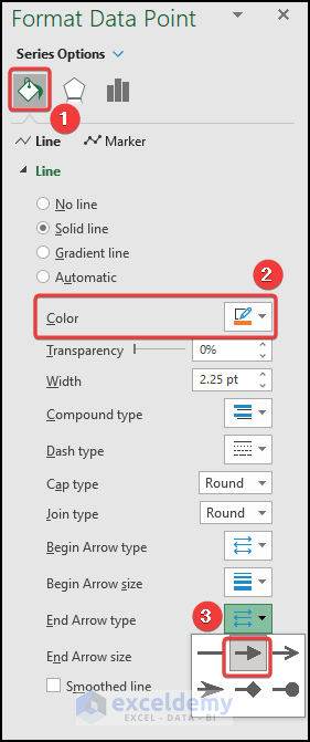
• Choose a color. Here, Orange.
• Specify the End Arrow type as shown below.

This is the output.

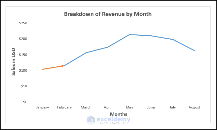
• Follow the same procedure for the other data points.
  This is the output.

Practice Section

Practice here.

Download Practice Workbook

Download the practice workbook.