Creating a Timeline Filter in Excel

Image by Editor
 

A Timeline filter in Excel is a visual tool specifically designed to filter data by date ranges. It allows users to easily navigate through different periods such as years, quarters, months, and days. It is especially useful when working with large datasets that contain date-related data like sales records, invoices, orders, etc.

In this tutorial, we will show how to create a Timeline in Excel.

Let’s consider a sample sales dataset that spans two years to show how to create and use timeline filters in Excel.

Step 1: Create an Excel Table

Timeline filters require data formatted as an Excel Table.

• Open Excel and load your dataset.
• Select your entire data range (including headers).
• Go to the Insert tab >> select Table or press CTRL+T.
• In the dialog box that appears >> select My table has headers.
• Click OK.

Excel Tables automatically expand when new data is added and maintain consistent formulas and formatting. They’re also required to use timeline filters.

Step 2: Create a PivotTable

Timeline filters work with tables and PivotTables. Let’s create a PivotTable to insert a timeline.

• Click anywhere within your Excel Table.
• Go to the Insert tab >> select PivotTable.
• In the dialog box:
  • Make sure the correct range is selected.
  • Choose whether to place the PivotTable in a new worksheet or an existing one.
  • Select New Worksheet as the placement (recommended).
  • Click OK.
• A new PivotTable will be created on a new worksheet, along with the PivotTable Fields pane.

Step 3: Set Up Your PivotTable

Let’s configure the PivotTable to analyze our sales data effectively.

• In the PivotTable Fields pane:
  • Drag the Region to the Rows section.
  • Drag the Product to the Columns section.
  • Drag Sales Amount to the Values section.

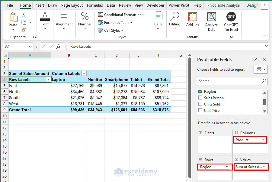
This makes the PivotTable ready for applying a timeline filter. We can now see overall sales patterns by region and product, but we don’t yet have a way to easily analyze how these patterns change over time.

Step 4: Add a Timeline Filter

Now insert the timeline filter.

• Click anywhere inside your PivotTable.
• Go to the PivotTable Analyze tab >> select Insert Timeline.
• In the dialog box, check the Date field.
• Click OK.

A timeline filter will appear on your worksheet. By default, it will show the entire order date range of your data. Now, this visual timeline interface will allow you to filter your data dynamically by different periods.

Step 5: Use Timeline Filter for Basic Analysis

Let’s explore how to use the timeline filter for basic analysis.

• Select a time level from the dropdown in the Timeline: Years, Quarters, Months, or Days.
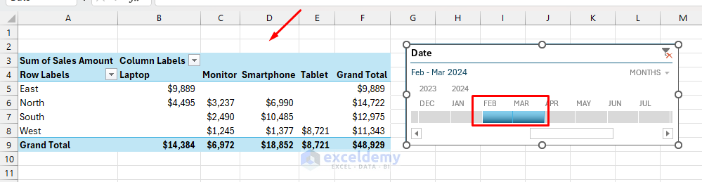
• Click the dropdown in the upper right corner of the timeline to change the time level to Months.
• Click on February 2024 in the timeline to filter your PivotTable to show only February 2024 data.

• Click and drag across February 2024 to March 2024 to select a range of months.
• PivotTable will update to include both months.

• Switch the timeline view to Quarters by clicking the dropdown in the upper right.
• Click on Q1 for 2024 to see the entire first quarter’s data.

You can quickly filter your data by different time periods and time levels (days, months, quarters, years) using the timeline filter.

Step 6: Customize Timeline Filter

Let’s improve the appearance and functionality of the timeline.

• Click on the timeline to select it.
• Go to the Timeline tab.
• You can now:
  • Change the Timeline Caption from Date to something more descriptive, like Sales Period.
  • Select different Timeline Styles from the gallery.
  • Click the More button to see additional options.
• Try changing the style to a more vibrant color scheme that matches your company branding.

You can resize, move, or format the Timeline as needed:

• To resize, click and drag from the corners.
• To move, click and drag the title bar.
• To clear filter, click the small funnel icon on the timeline.

A well-designed timeline filter not only looks more professional but also makes it easier for users to understand and interact with the data.

Step 7: Add Additional Context with PivotTable Filters

Let’s enhance our analysis by adding more dimensions.

• Keep your timeline filter as is, but add another field to your PivotTable:
  • Drag the Sales Person to the Filters area at the top of the PivotTable.
• Click the dropdown in the Sales Person filter >> select John.
• PivotTable will show only John’s sales for the selected time periods.

You can try filtering for different salespeople while maintaining your timeline selection. By combining timeline filters with standard PivotTable filters, you can create multi-dimensional analyses that provide deeper insights.

Step 9: Create a PivotChart Connected to Timeline Filter

Let’s visualize the time-based data.

• Select the PivotTable.
• Go to the PivotTable Analyze tab >> select PivotChart.
• Select a Clustered Column chart >> click OK.

• A PivotChart will appear, showing data visually.
• Notice that when you interact with the timeline filter, both your PivotTable and PivotChart update simultaneously.

Adding a visual representation makes it easier to spot trends and patterns that might be less obvious in tabular format.

Step 10: Connect Multiple PivotTables to One Timeline

If you want to analyze your data in different ways simultaneously.

• Create another PivotTable using the same data source (your Excel Table).
• Configure it differently.
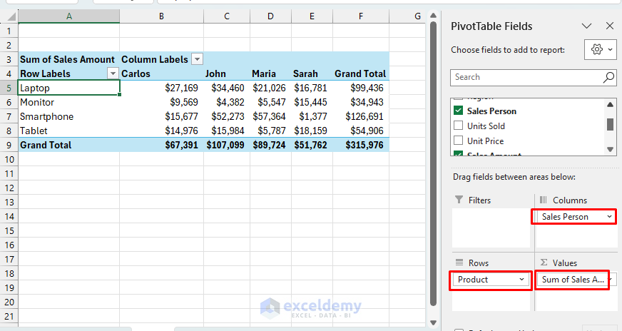
  • Drag the Product in the rows section.
  • Drag the Sales Person to the columns section.
  • Drag Sales Amount to the Values section.

• Right-click on the existing timeline filter and select Report Connections.

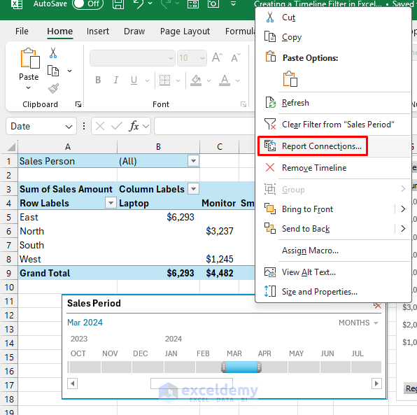
• Check the box for new PivotTable2 >> click OK.
• Now, when you use the timeline filter, both PivotTables will update in sync.

Test Interactivity:

• Select time level Years >> select year 2023.

• Select Year 2024.

The Timeline feature is applied to all the existing tables and charts. This technique allows you to maintain consistent time filters across multiple analyses, saving time and ensuring consistency.

Troubleshoot Common Timeline Issues

If you encounter any issues with your timeline filter, here are some common solutions.

• Timeline option greyed out:
  • Ensure your data contains at least one properly formatted date field.
  • Verify you’re using Excel 2013 or newer.
  • Check that your PivotTable is properly created.
• Timeline not filtering correctly:
  • Confirm your date field is properly formatted as dates in your source data.
  • Try recreating the PivotTable and timeline.
• Dates not appearing as expected:
  • Check your date formats in the source data.
  • Make sure there are no text values in your date column.

Conclusion

Timeline filters in Excel provide a powerful and intuitive way to analyze time-based data. By mastering this feature, you can quickly filter and visualize data across different time periods, making your data analysis more efficient and insightful. Remember that timeline filters are most effective when used with well-structured data and thoughtfully designed PivotTables. With practice, you’ll be able to leverage this feature to gain valuable insights from your time-based data.