How to Create a Cash Flow Projection Template in Excel

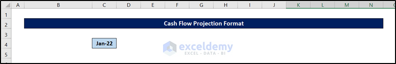
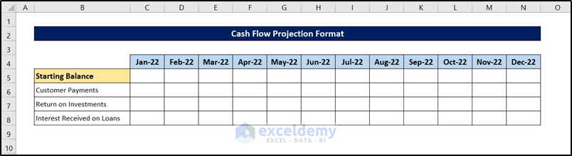
Step 1 – Record Time Intervals

• Enter the first time period at the top of the template.

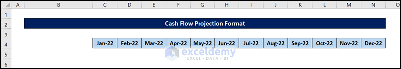
• Use the Autofill Tool and drag to fill in the other time periods.

Read More: How to Create Cash Flow Projection for 12 Months in Excel

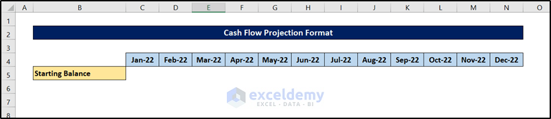
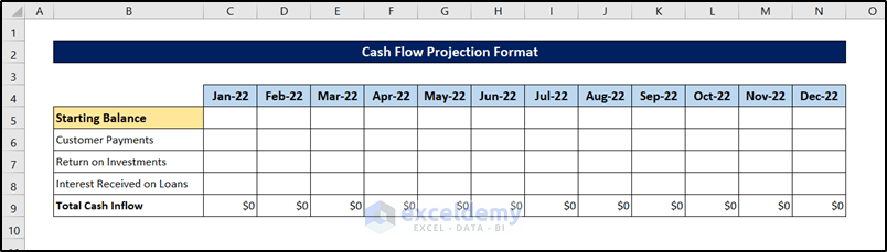
Step 2 – Create a Section for the Starting Balance

• Select an appropriate cell and label it “Starting Balance”.

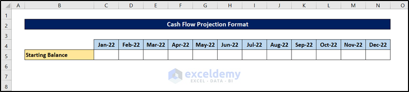
• Format the data cells for each period.

Read More: How to Create a Real Estate Cash Flow Model in Excel

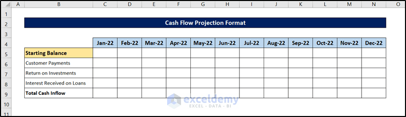
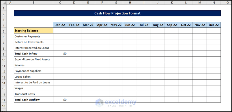
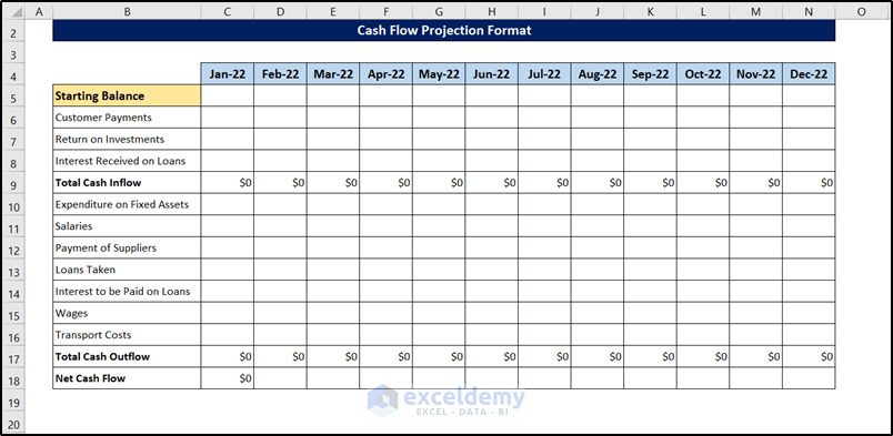
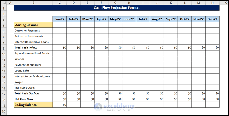
Step 3 – Add All Cash Inflow Sources

• Add rows for and label all the Cash Inflow sources you will record data for later.

Read More: How to Create a Retirement Cash Flow Calculator in Excel

Step 4 – Set Up Cash Inflow Totals

• Add a row to total the Cash Inflow for each period.

• Select the first Cash Inflow total (cell C9 in this example) and enter the following formula:

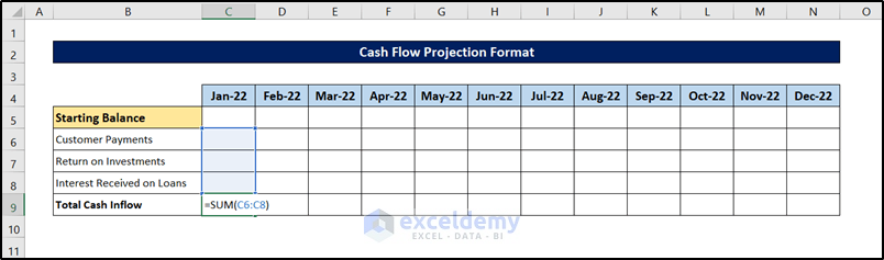
Press Enter.

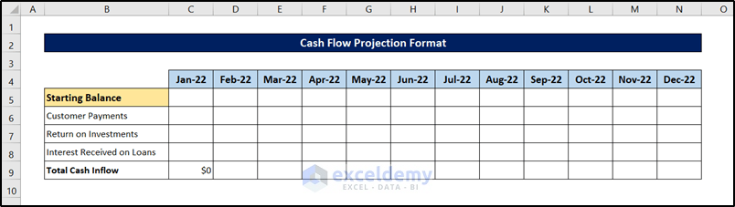
• Use the Autofill Tool and drag to fill in the other cells in the row.

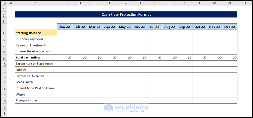
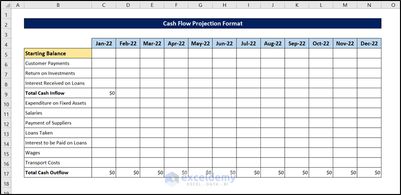
Step 5 – Add All Cash Outflow Sources

• Add rows for and label all of the Cash Outflow sources.

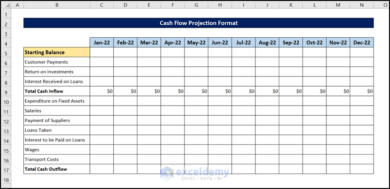
Step 6 – Set Up Cash Outflow Totals

• Add a row to total the Cash Outflow for each period.

• Select the first Cash Outflow total (C17 in this example) and enter the following formula:

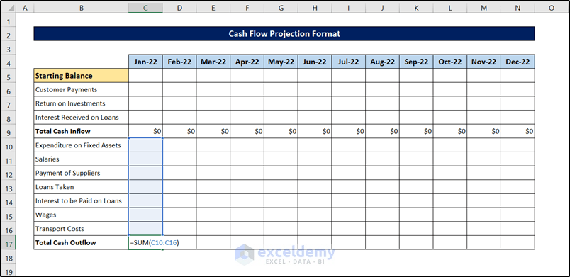
• Press Enter.

• Use the Autofill Tool and drag to fill in the other cells in the row.

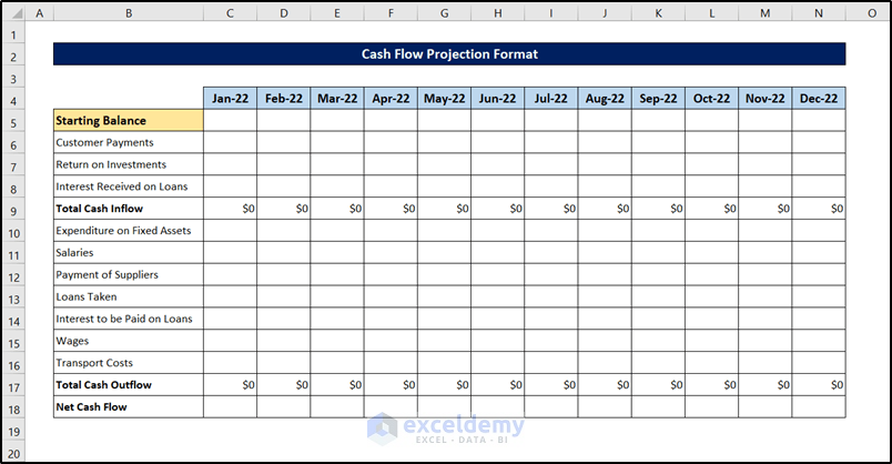
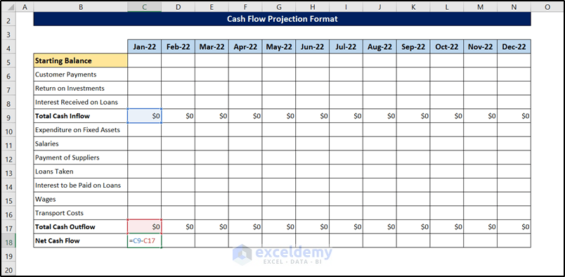
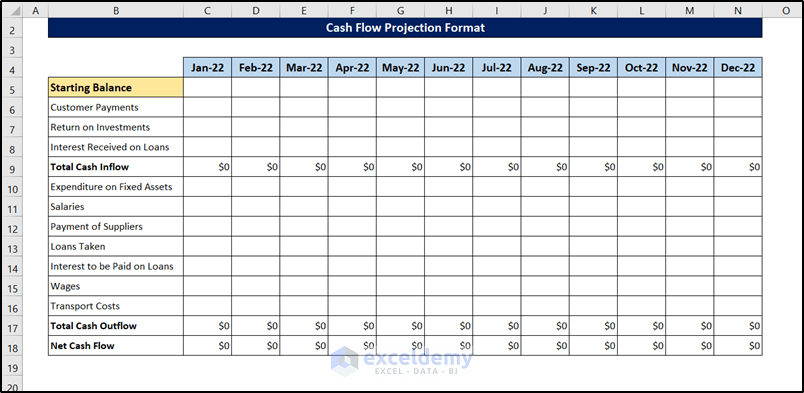
Step 7 – Add and Set Up Net Cash Flow Totals

• Add a row for Net Cash Flow.

• Select the first Net Cash Flow total (C18 in this example) and enter the following formula:

• Press Enter.

• Use the Autofill Tool and drag to fill in the other cells in the row.

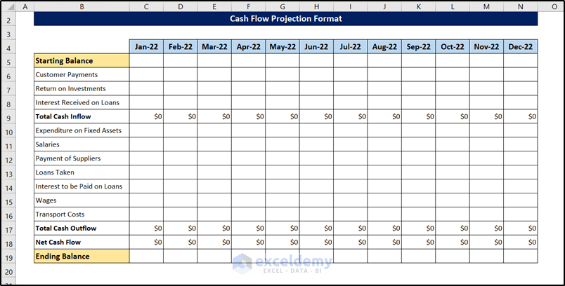
Step 8 – Add and Set Up Ending Balance Totals

• Add a row for Ending Balance.

• Select the first Ending Balance total (C19 in this example) and enter the following formula:

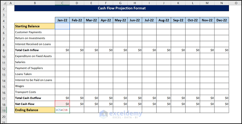
• Press Enter.

• Use the Autofill Tool and drag to fill in the other cells in the row.

Step 9 – Replicate the Starting Balance Formula

• Select the Starting Balance for the second period (Cell D5 in this example) and enter the following formula:

• Press Enter.

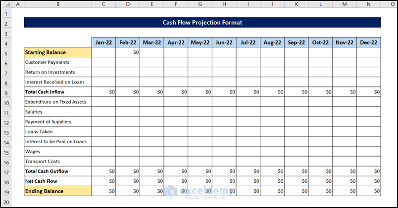
• Use the Autofill Tool and drag to fill in the other cells in the row.

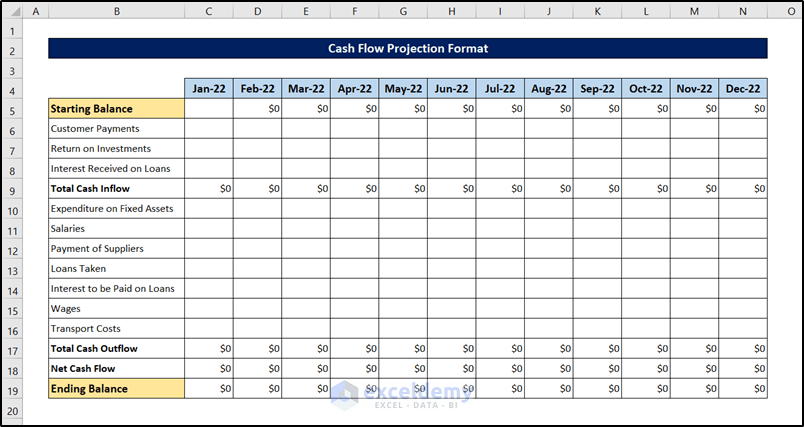
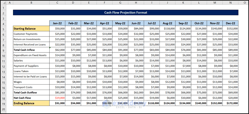
The Cash Flow Projection Template is complete.

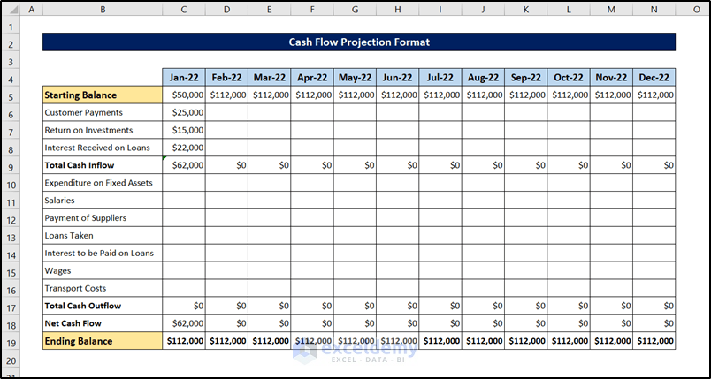
Step 10 – Verify the Template with Test Data

Enter a Starting Balance of $50000 for the initial time period.

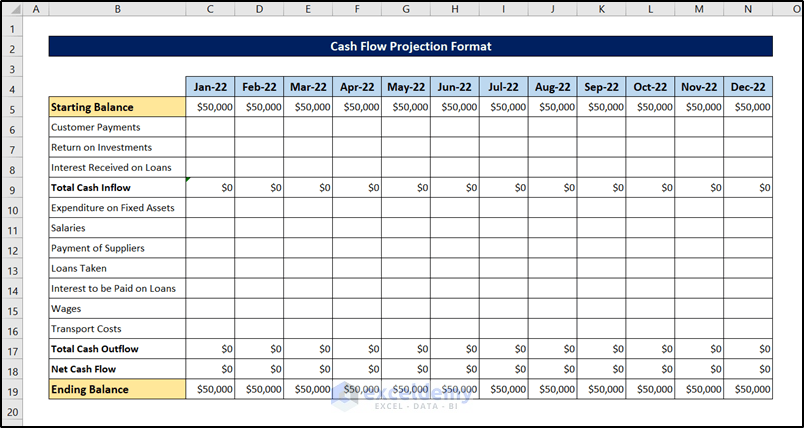
• Enter amounts for the Cash Inflow sources.
• Cash Inflow and Net Cash Flow totals should update automatically.

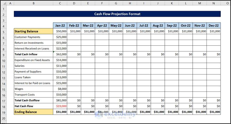
• Repeat for the Cash Outflow sources.
• Verify every cell in the first column has been updated.

• Repeat for the remaining periods to verify the formulas are all working properly.

Download Practice Workbook

You can download the workbook used for the demonstration from the link below. You can use it as your personal template too with some modifications.

Related Articles

• How to Create Investment Property Cash Flow Calculator in Excel
• How to Make a Restaurant Cash Flow Statement in Excel

<< Go Back to Cash Flow Template | Finance Template | Excel Templates