How to Calculate Weight Loss Percentage in Excel (5 Methods)

Suppose we have the dataset below of weight measurements taken every 15 days for 4 months, and we want to calculate the weight loss percentage for each consecutive date and over the whole period.

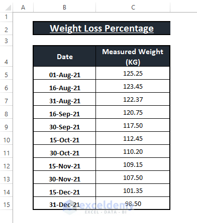
In this article, we’ll demonstrate 5 ways to calculate weight loss percentage using this dataset.

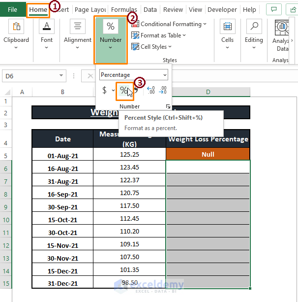
Before commencing with the methods, set the cell format to percentage, so that the percentage rather than fractions will be automatically displayed whenever the percentage is calculated. To do so:

• Highlight the cells.
• Go to the Home tab.
• Select Percentage from the Number section.

Method 1 – Calculate Weight Loss Percentage Using an Arithmetic Formula

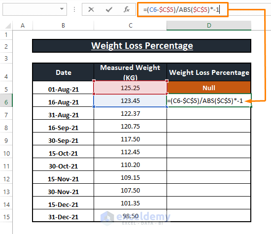
We can calculate the weight loss percentage with an arithmetic formula. Subtracting the initial weight from the next and then dividing by the initial weight results in the weight loss percentage between the two values.

Steps:

• Paste the below formula in any cell (eg D6):

The ABS function returns the absolute value of a number.

• Press Enter.

As the cells are already formatted in Percentage format, the result is displayed in percent.

• Drag the Fill Handle down to copy the formula to the rest of the cells below.

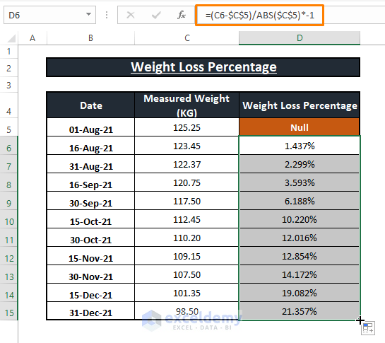
We have the weight loss percentages for each interval.

Method 2 – Using the MIN Function to Assign a Minimum Value in the Percentage Calculation

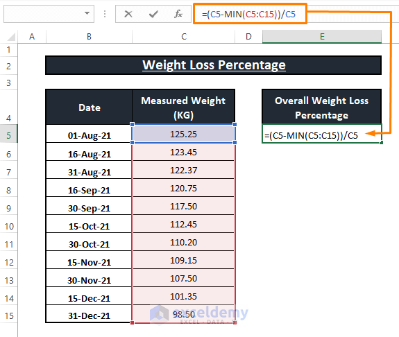
Suppose we want to find the overall weight loss over the full period. We’ll need to find the minimum weight within the range to use as the initial weight, which we’ll accomplish using the MIN function.

Steps:

• Enter the following formula in any blank cell (eg E5):

The MIN function fetches the minimum weight within the range C5:C15.

• Press ENTER to display the total weight loss percentage.

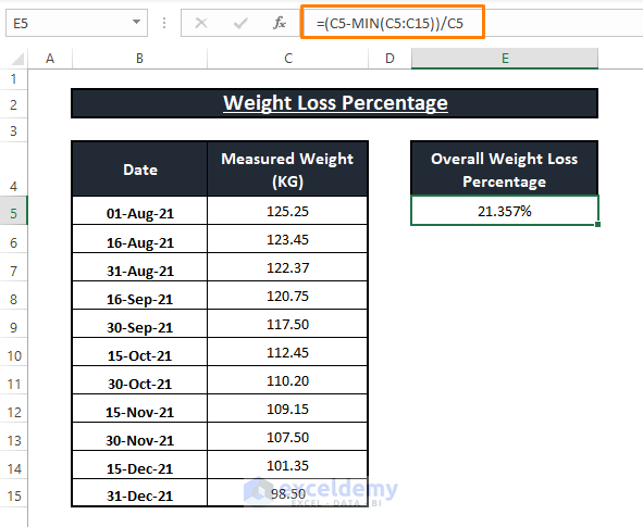
If the cells aren’t formatted in Percentage format, decimal values will appear instead of percentages.

Method 3 – Using the LOOKUP Function to Find the Final Value in the Percentage Calculation

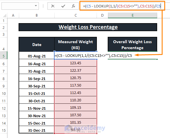
In a similar way to Method 2, we can use the LOOKUP function to find the last weight in the range to slot into our weight loss percentage formula.

Steps:

Enter the formula below in any cell (eg, E5):

In the LOOKUP function, 1 is the lookup_value, 1/(C5:C15<>””) is the lookup_vector, and C5:C15 is the result_vector.

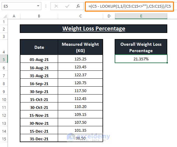
• Press ENTER to return the overall weight loss percentage.

Method 4 – Finding the Most Recent Value Using the OFFSET and COUNT Functions

We can use the OFFSET function to assign row and column numbers from which to find the most recent weight value for our formula.

Steps:

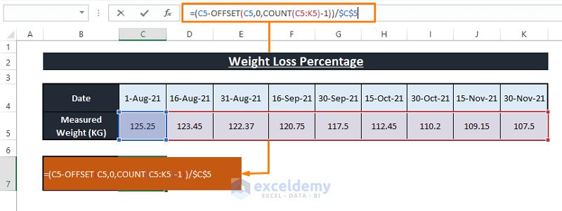
• Enter the following formula in any empty cell:

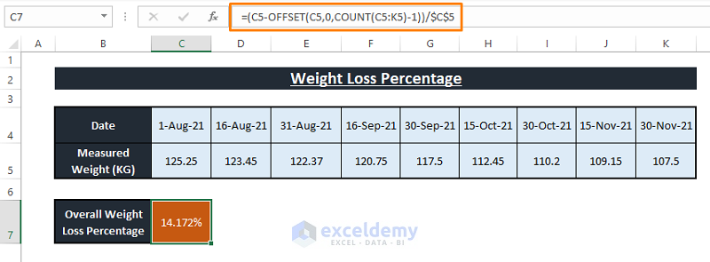
In the formula, C5 is the reference, 0 is the rows, and COUNT(C5:K5)-1 is the cols. The OFFSET portion of the formula fetches the rightmost weight value to deduct from the initial value.

• Press ENTER to return the overall percentage weight loss considering the rightmost value as the most recent weight value.

The OFFSET formula is specially used for horizontal series. We could also use the typical Arithmetic Formula in this case, however it becomes increasingly inefficient as the dataset’s size grows.

Method 5 – Using INDEX-COUNT to Fetch the Last Value 

Similarly to the last method, we can use the INDEX function to insert the last row value from the given range into our weight loss percentage formula.

Steps:

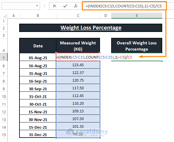
• Enter the following formula in any cell:

The INDEX portion of the formula declares C5:C15 as an array, COUNT(C5:C15) as row_num, and 1 as column_num. The COUNT function passes the row_num of the given range (C5:C15).

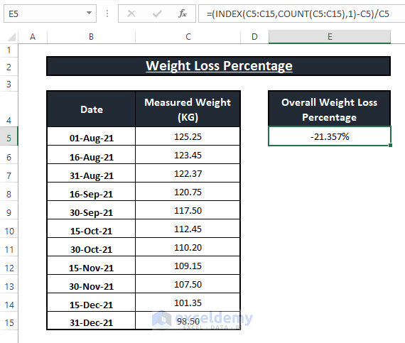
• Press ENTER.

The overall weight loss percentage will be displayed with a minus (–) sign, which indicates a weight reduction occurred over the observed period of time.

Download Practice Workbook

<< Go Back to Weight Loss | Formula List | Learn Excel