Excel has one of the best usages in statistics. Average Deviation is an important term in statistics that can be directly measured in Excel with the AVEDEV function. In this article, we will discuss and show you some examples of the AVEDEV function in Excel.
Introduction to AVEDEV Function in Excel
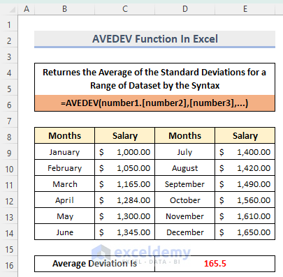
The AVEDEV function stands for Average Deviation. That means it will calculate the average deviation from a bunch of data. In any data set, deviations between numerical values are common. The average deviation gives the idea of how close those data are in the given range.
Syntax:
The syntax of AVEDEV function is below:
=AVEDEV(number1,[number2],[number3],[number4],...)Arguments:
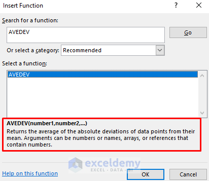
AVEDEV function can have up to 255 arguments at max. But there should be at least 1 argument. The first argument is defined by number1 in the formula. The rest of the arguments are not mandatory. They are represented as [number2], [number3], [number4] and so on. It’s mandatory. All the arguments can be discrete numbers, names, arrays or other cell references that contain numeric values.
| ARGUMENT | REQUIREMENT | EXPLANATION |
|---|---|---|
| number1 | Required | Any numeric value. |
| [number2],[number3],… | Optional | Next numeric values. These are optional. |
Return Value:
Returns a numeric value that represents the average of the absolute deviations of data points from their mean. If there is no difference between any of the data, meaning all the data has the same numeric value, the AVEDEV function will return 0.
Available In:
The AVEDEV function is available from Excel 2003 to all later versions. But the Excel 2003 version has only 30 arguments while the later versions have 255.
Using the AVEDEV Function in Excel: 2 Simple Examples
Here are the two different examples that show the different uses of the AVEDEV function in Excel. The examples are explained below.
Example 1: Basic Use of AVEDEV Function
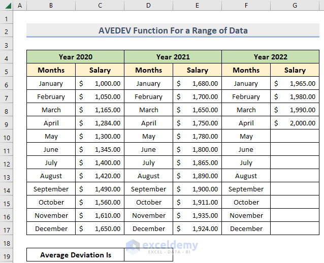
In this example, we will use data ranges as arguments to get the average deviation. The steps are below.
🔶 Steps:
- At first, we will need a data set where we can use the AVEDEV function. Below, we attached a sample dataset that can be used. Here, we have the salary of an employee over time. We want to find the average deviation of his/her Salary.
- Next, we will click on the cell where we want the average deviation. In our case, the cell is D19.
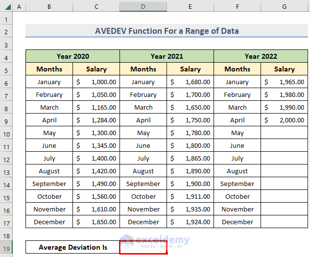
- Then, write the following formula in the cell and click Enter.
=AVEDEV(C6:C17,E6:E17,G6:G17)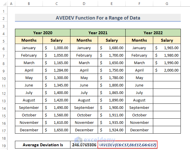
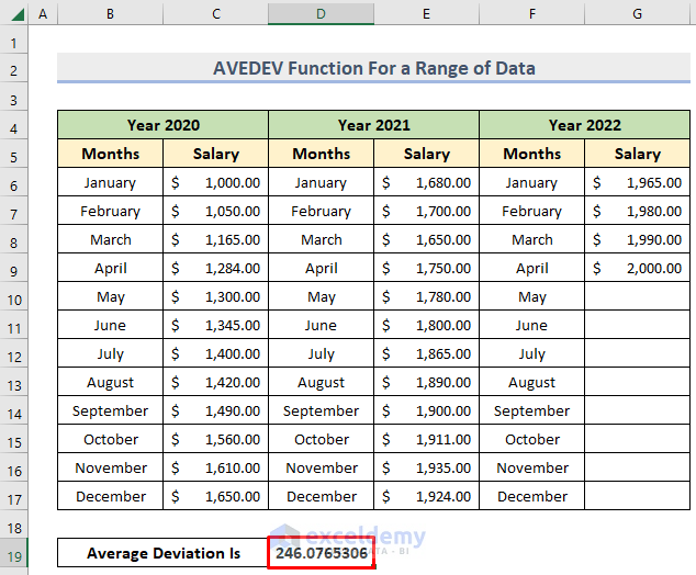
- Finally, we will get the result like the following.
Example 2: Use of AVEDEV Function to Find Average Deviation of Discrete Data
In this example, we will use discrete data to find the average deviation for the small data set below.
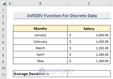
The steps are below.
🔶 Steps:
- First, select the destination cell. In our case the cell is C11.
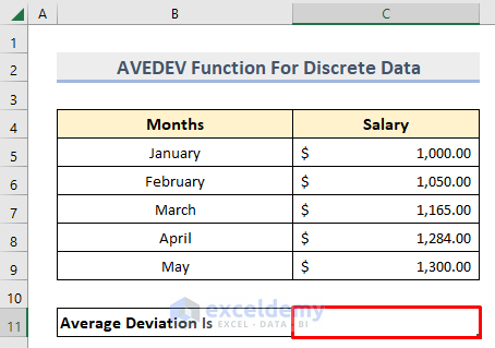
- Next, we will directly write the AVEDEV function with the data one by one like the following formula.
=AVEDEV(1000,1050,1165,1284,1300)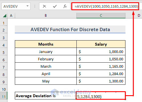
- Then, press Enter to get the result.

Things to Remember
- For AVEDEV function to work, all the input arguments must be numerical values.
- If all the inputs carry the same numeric value, the function will return 0.
- Again, the number of arguments is bound to 255. For Excel 2003 the number is 30.
- Lastly, if input arguments carry units, the AVEDEV function will take that into account and change accordingly.
Download Practice Workbook
Download the following workbook that we used to write this article so that you can practice along with it while reading the article.
Conclusion
That is all the necessary information and applications that you need to know about the AVEDEV function in Excel. If you’re still having trouble with any of these examples or have any queries about the function, let us know in the comments. Our team is ready to answer all of your questions.
<< Go Back to Excel Functions | Learn Excel
Get FREE Advanced Excel Exercises with Solutions!
